DS4000 Rigol Waveform Examples
Scott Prahl
March 2021
This notebook illustrates shows how to extract signals from a .wfm file created by a the Rigol DS4000 scope. It also validates that the process works by comparing with .csv and screenshots.
Two different .wfm files are examined one for the DS4022 scope and one for the DS4024 scope. The accompanying .csv files seem to have t=0 in the zero in the center of the waveform.
If RigolWFM is not installed, uncomment the following cell (i.e., delete the #) and run (shift-enter)
[1]:
#!pip install --user RigolWFM
[2]:
import numpy as np
import matplotlib.pyplot as plt

try:
    import RigolWFM.wfm as rigol
except ModuleNotFoundError:
    print('RigolWFM not installed. To install, uncomment and run the cell above.')
    print('Once installation is successful, rerun this cell again.')

repo = "https://github.com/scottprahl/RigolWFM/raw/master/wfm/"
A list of Rigol scopes that should have the same file format is:
[3]:
print(rigol.DS4000_scopes)
['4', '4000', 'DS4000', 'DS4054', 'DS4052', 'DS4034', 'DS4032', 'DS4024', 'DS4022', 'DS4014', 'DS4012', 'MSO4054', 'MSO4052', 'MSO4034', 'MSO4032', 'MSO4024', 'MSO4022', 'MSO4014', 'MSO4012']
DS4022 Waveform
Look at a screen shot
Start with a .wfm file from a Rigol DS4022 scope. It should looks something like this

Import the .wfm data
[4]:
# raw=true is needed because this is a binary file
name = "DS4022-A.wfm"
wfm_filename = repo + name + "?raw=true"

w = rigol.Wfm.from_url(wfm_filename, '4000')
downloading 'https://github.com/scottprahl/RigolWFM/raw/master/wfm/DS4022-A.wfm?raw=true'
First a textual description.
[5]:
description = w.describe()
print(description)
    General:
        File Model   = wfm4000
        User Model   = 4000
        Parser Model = wfm4000
        Firmware     = 00.02.03.00.03
        Filename     = DS4022-A.wfm
        Channels     = [1, 2, 3, 4]

     Channel 1:
         Coupling =       DC
            Scale =    50.00  V/div
           Offset =     0.00  V
            Probe =      10X
         Inverted =    False

        Time Base =    1.000 µs/div
           Offset =  500.000 ns
            Delta =    2.000 ns/point
           Points =     7000

         Count    = [        1,        2,        3  ...      6999,     7000]
           Raw    = [      215,      222,      227  ...        20,       20]
           Times  = [-6.500 µs,-6.498 µs,-6.496 µs  ...  7.498 µs, 7.500 µs]
           Volts  = [137.50  V,148.44  V,156.25  V  ... -167.19  V,-167.19  V]

     Channel 2:
         Coupling =       DC
            Scale =   200.00  V/div
           Offset =     0.00  V
            Probe =     100X
         Inverted =    False

        Time Base =    1.000 µs/div
           Offset =  500.000 ns
            Delta =    2.000 ns/point
           Points =     7000

         Count    = [        1,        2,        3  ...      6999,     7000]
           Raw    = [      127,      127,      127  ...       127,      127]
           Times  = [-6.500 µs,-6.498 µs,-6.496 µs  ...  7.498 µs, 7.500 µs]
           Volts  = [ -0.00  V, -0.00  V, -0.00  V  ...  -0.00  V, -0.00  V]

     Channel 3:
         Coupling =       DC
            Scale =    50.00  V/div
           Offset =     0.00  V
            Probe =      10X
         Inverted =    False

        Time Base =    1.000 µs/div
           Offset =  500.000 ns
            Delta =    2.000 ns/point
           Points =     7000

         Count    = [        1,        2,        3  ...      6999,     7000]
           Raw    = [       65,       57,       49  ...       236,      236]
           Times  = [-6.500 µs,-6.498 µs,-6.496 µs  ...  7.498 µs, 7.500 µs]
           Volts  = [-96.88  V,-109.38  V,-121.88  V  ... 170.31  V,170.31  V]

     Channel 4:
         Coupling =       DC
            Scale =   200.00  V/div
           Offset =     0.00  V
            Probe =     100X
         Inverted =    False

        Time Base =    1.000 µs/div
           Offset =  500.000 ns
            Delta =    2.000 ns/point
           Points =     7000

         Count    = [        1,        2,        3  ...      6999,     7000]
           Raw    = [      127,      127,      127  ...       128,      127]
           Times  = [-6.500 µs,-6.498 µs,-6.496 µs  ...  7.498 µs, 7.500 µs]
           Volts  = [ -0.00  V, -0.00  V, -0.00  V  ...   6.25  V, -0.00  V]
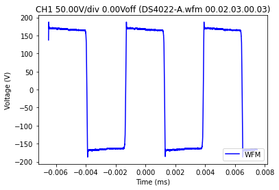
Now for the actual signal
[6]:
toff=0.05
ch=w.channels[0]
plt.title("CH%d %.2fV/div %.2fVoff (%s %s)" % (1,ch.volt_per_division, ch.volt_offset, w.basename, w.firmware))
plt.plot(ch.times*1e3,ch.volts, color='blue', label='WFM')

plt.legend(loc='lower right')
plt.xlabel("Time (ms)")
plt.ylabel("Voltage (V)")

plt.show()
[7]:
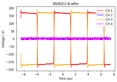
# Note that CH3 and CH4 are both effectively zero, just displaced in the display graph above
w.plot()
plt.show()
DS4024 Waveform
Start with importing the .csv data
[8]:
filename = "DS4024-A.csv"
csv_filename = repo + filename

csv_data = np.genfromtxt(csv_filename, delimiter=',', skip_header=2).T

# need to do this separately because only the start and increment is given in the csv file
time = csv_data[0] * 2.000000e-06 - 1.400000e-03
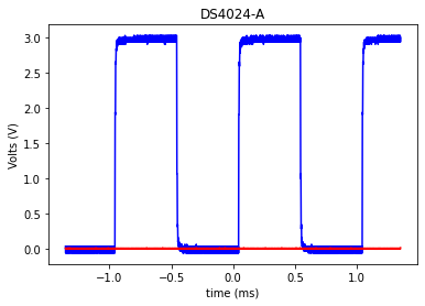
Plot the .csv data
[9]:
plt.plot(time*1000,csv_data[1], color='blue')
plt.plot(time*1000,csv_data[2], color='red')
plt.xlabel("time (ms)")
plt.ylabel("Volts (V)")
plt.title("DS4024-A")
plt.show()
Import the .wfm data
[10]:
# raw=true is needed because this is a binary file
name = "DS4024-A.wfm"
wfm_filename = repo + name + "?raw=true"

w = rigol.Wfm.from_url(wfm_filename, '4')
downloading 'https://github.com/scottprahl/RigolWFM/raw/master/wfm/DS4024-A.wfm?raw=true'
Now describe the .wfm data
[11]:
print(w.describe())
    General:
        File Model   = wfm4000
        User Model   = 4
        Parser Model = wfm4000
        Firmware     = 00.02.03.02.00
        Filename     = DS4024-A.wfm
        Channels     = [1, 2]

     Channel 1:
         Coupling =       DC
            Scale =     1.00  V/div
           Offset =  -576.00 mV
            Probe =       1X
         Inverted =    False

        Time Base =  200.000 µs/div
           Offset =  100.000 µs
            Delta =    4.000 ns/point
           Points =   700000

         Count    = [        1,        2,        3  ...    699999,   700000]
           Raw    = [      109,      109,      109  ...       205,      206]
           Times  = [-1.300 ms,-1.300 ms,-1.300 ms  ...  1.500 ms, 1.500 ms]
           Volts  = [ 13.50 mV, 13.50 mV, 13.50 mV  ...   3.01  V,  3.04  V]

     Channel 2:
         Coupling =       DC
            Scale =   200.00 mV/div
           Offset =     0.00  V
            Probe =       1X
         Inverted =    False

        Time Base =  200.000 µs/div
           Offset =  100.000 µs
            Delta =    4.000 ns/point
           Points =   700000

         Count    = [        1,        2,        3  ...    699999,   700000]
           Raw    = [      126,      127,      127  ...       127,      127]
           Times  = [-1.300 ms,-1.300 ms,-1.300 ms  ...  1.500 ms, 1.500 ms]
           Volts  = [ -6.25 mV, -0.00  V, -0.00  V  ...  -0.00  V, -0.00  V]
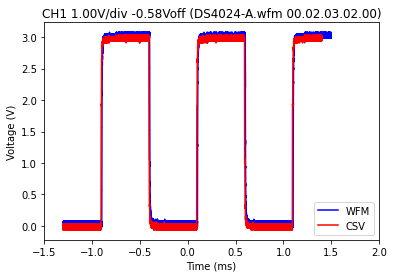
Finally compare the .wfm data to the .csv data
[12]:
toff=0.05
ch=w.channels[0]
plt.title("CH%d %.2fV/div %.2fVoff (%s %s)" % (1,ch.volt_per_division, ch.volt_offset, w.basename, w.firmware))
plt.plot(ch.times*1e3,ch.volts, color='blue', label='WFM')

plt.plot(time*1e3+toff,csv_data[1], color='red', label='CSV')
plt.legend(loc='lower right')
plt.xlabel("Time (ms)")
plt.ylabel("Voltage (V)")
plt.xlim(-1.5,2)

plt.show()
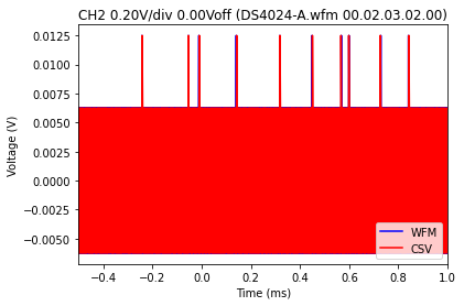
[13]:
toff=0.0565

ch=w.channels[1]
plt.title("CH%d %.2fV/div %.2fVoff (%s %s)" % (2,ch.volt_per_division, ch.volt_offset, w.basename, w.firmware))
plt.plot(ch.times*1e3,ch.volts, color='blue', label='WFM')

plt.plot(time*1e3+toff,csv_data[2], color='red', label='CSV')
plt.legend(loc='lower right')
plt.xlabel("Time (ms)")
plt.ylabel("Voltage (V)")
plt.xlim(-0.5,1.0)
#plt.ylim(-0.02,0.02)
plt.show()
[ ]: