DS2000 Rigol Waveform Examples
Scott Prahl
March 2021
This notebook demonstrates extracting signals from .wfm files created by Rigol DS2000 oscilloscopes. It also validates that the process works by comparing with .csv and screenshots.
If RigolWFM is not installed, uncomment the following cell (i.e., delete the #) and run (shift-enter)
[1]:
#!pip install --user RigolWFM
[2]:
import numpy as np
import matplotlib.pyplot as plt

try:
    import RigolWFM.wfm as rigol
except ModuleNotFoundError:
    print('RigolWFM not installed. To install, uncomment and run the cell above.')
    print('Once installation is successful, rerun this cell again.')

repo = "https://github.com/scottprahl/RigolWFM/raw/master/wfm/"

def read_rigol_csv(name):
    csv_data = np.genfromtxt(name, delimiter=',', skip_header=2).T
    lines = len(csv_data[0])
    header=np.genfromtxt(name, delimiter=',', skip_footer=lines, names=True)
    offset, scale = header['Start'], header['Increment']
    csv_data[0] = offset + scale * csv_data[0]
    return csv_data
A list of Rigol scopes in the DS2000 family is:
[3]:
print(rigol.DS2000_scopes)
['2', '2000', 'DS2000', 'DS2072A', 'DS2102A', 'MSO2102A', 'MSO2102A-S', 'DS2202A', 'MSO2202A', 'MSO2202A-S', 'DS2302A', 'MSO2302A', 'MSO2302A-S']
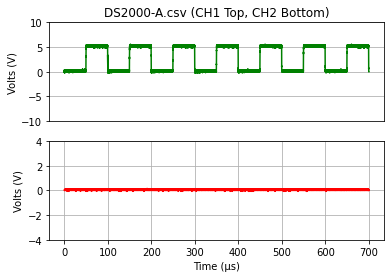
DS2000-A
Look at a screen shot
Start with a .wfm file from a Rigol DS2000 scope. It should look something like this

Look at the data in the .csv file
First let’s look at plot of the data from the corresponding .csv file. Unfortunately this wfm file did not come with a .csv file generated by the Rigol oscilloscope. Instead, the .csv was generated by RigolWFM and verifies that the .csv generation matches that expected.
[4]:
filename = "DS2000-A.csv"

csv_data = np.genfromtxt(repo+filename, delimiter=',', skip_header=2).T

plt.subplot(211)
plt.plot(csv_data[0]*1e6,csv_data[1], color='green')
plt.title(filename + " (CH1 Top, CH2 Bottom)")
plt.ylabel("Volts (V)")
plt.ylim(-10,10)
plt.grid(True)
plt.xticks([])

plt.subplot(212)
plt.plot(csv_data[0]*1e6,csv_data[2], color='red')
plt.xlabel("Time (µs)")
plt.ylabel("Volts (V)")
plt.grid(True)
plt.ylim(-4,4)

plt.show()
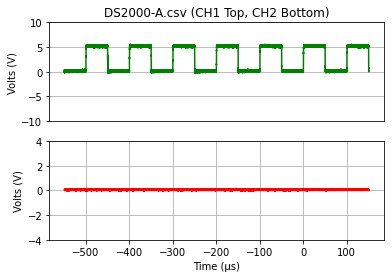
Now for the .wfm data
First a textual description.
[5]:
# raw=true is needed because this is a binary file
wfm_url = repo + "DS2000-A.wfm" + "?raw=true"
w = rigol.Wfm.from_url(wfm_url, '2000')

description = w.describe()
print(description)
downloading 'https://github.com/scottprahl/RigolWFM/raw/master/wfm/DS2000-A.wfm?raw=true'
    General:
        File Model   = wfm2000
        User Model   = 2000
        Parser Model = wfm2000
        Firmware     = 00.03.00.01.03
        Filename     = DS2000-A.wfm
        Channels     = [1, 2]

     Channel 1:
         Coupling =       DC
            Scale =     5.00  V/div
           Offset =     0.00  V
            Probe =      10X
         Inverted =    False

        Time Base =   50.000 µs/div
           Offset = -199.200 µs
            Delta =    1.000 ns/point
           Points =   700000

         Count    = [        1,        2,        3  ...    699999,   700000]
           Raw    = [      128,      127,      129  ...       128,      128]
           Times  = [-549.200 µs,-549.199 µs,-549.198 µs  ... 150.799 µs,150.800 µs]
           Volts  = [200.00 mV, -0.00  V,400.00 mV  ... 200.00 mV,200.00 mV]

     Channel 2:
         Coupling =       DC
            Scale =     2.00  V/div
           Offset =    -6.00  V
            Probe =      10X
         Inverted =    False

        Time Base =   50.000 µs/div
           Offset = -199.200 µs
            Delta =    1.000 ns/point
           Points =   700000

         Count    = [        1,        2,        3  ...    699999,   700000]
           Raw    = [       53,       52,       53  ...        52,       53]
           Times  = [-549.200 µs,-549.199 µs,-549.198 µs  ... 150.799 µs,150.800 µs]
           Volts  = [ 80.00 mV,476.84 nV, 80.00 mV  ... 476.84 nV, 80.00 mV]
[6]:
ch = w.channels[0]
plt.subplot(211)
plt.plot(ch.times*1e6, ch.volts, color='green')
plt.title(filename + " (CH1 Top, CH2 Bottom)")
plt.ylabel("Volts (V)")
plt.ylim(-10,10)
plt.grid(True)
plt.xticks([])

ch = w.channels[1]
plt.subplot(212)
plt.plot(ch.times*1e6, ch.volts, color='red')
plt.xlabel("Time (µs)")
plt.ylabel("Volts (V)")
plt.ylim(-4,4)
plt.grid(True)

plt.show()
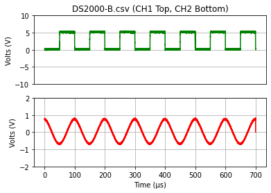
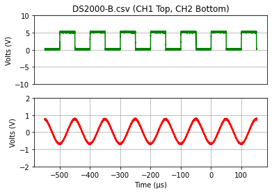
DS2000-B

First the .csv data
Let’s look at what the accompanying .csv data looks like.
[7]:
filename = "DS2000-B.csv"

# unfortunately this csv file was generated by RigolWFM and by not the scope itself
csv_data = np.genfromtxt(repo+filename, delimiter=',', skip_header=2).T

plt.subplot(211)
plt.plot(csv_data[0]*1e6,csv_data[1], color='green')
plt.title(filename + " (CH1 Top, CH2 Bottom)")
plt.ylabel("Volts (V)")
plt.ylim(-10,10)
plt.grid(True)
plt.xticks([])

plt.subplot(212)
plt.plot(csv_data[0]*1e6,csv_data[2], color='red')
plt.xlabel("Time (µs)")
plt.ylabel("Volts (V)")
plt.grid(True)
plt.ylim(-2,2)

plt.show()
Now for the wfm data
First let’s have look at the description of the internal file structure. We see that only channel 1 has been enabled.
[8]:
# raw=true is needed because this is a binary file
wfm_url = repo + "DS2000-B.wfm" + "?raw=true"

w = rigol.Wfm.from_url(wfm_url, 'DS2000')
description = w.describe()
print(description)
downloading 'https://github.com/scottprahl/RigolWFM/raw/master/wfm/DS2000-B.wfm?raw=true'
    General:
        File Model   = wfm2000
        User Model   = DS2000
        Parser Model = wfm2000
        Firmware     = 00.03.00.01.03
        Filename     = DS2000-B.wfm
        Channels     = [1, 2]

     Channel 1:
         Coupling =       DC
            Scale =     5.00  V/div
           Offset =    -5.00  V
            Probe =      10X
         Inverted =    False

        Time Base =   50.000 µs/div
           Offset = -199.200 µs
            Delta =    1.000 ns/point
           Points =   700000

         Count    = [        1,        2,        3  ...    699999,   700000]
           Raw    = [      103,      102,      103  ...       103,      103]
           Times  = [-549.200 µs,-549.199 µs,-549.198 µs  ... 150.799 µs,150.800 µs]
           Volts  = [200.00 mV,  0.00  V,200.00 mV  ... 200.00 mV,200.00 mV]

     Channel 2:
         Coupling =       DC
            Scale =     1.00  V/div
           Offset =    -3.00  V
            Probe =      10X
         Inverted =    False

        Time Base =   50.000 µs/div
           Offset = -199.200 µs
            Delta =    1.000 ns/point
           Points =   700000

         Count    = [        1,        2,        3  ...    699999,   700000]
           Raw    = [       71,       72,       71  ...        71,       72]
           Times  = [-549.200 µs,-549.199 µs,-549.198 µs  ... 150.799 µs,150.800 µs]
           Volts  = [760.00 mV,800.00 mV,760.00 mV  ... 760.00 mV,800.00 mV]
[9]:
ch = w.channels[0]
plt.subplot(211)
plt.plot(ch.times*1e6, ch.volts, color='green')
plt.title(filename + " (CH1 Top, CH2 Bottom)")
plt.ylabel("Volts (V)")
plt.ylim(-10,10)
plt.grid(True)
plt.xticks([])

ch = w.channels[1]
plt.subplot(212)
plt.plot(ch.times*1e6, ch.volts, color='red')
plt.xlabel("Time (µs)")
plt.ylabel("Volts (V)")
plt.ylim(-2,2)
plt.grid(True)

plt.show()
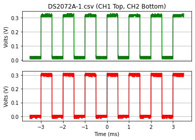
DS2072A-1
Look at a screen shot
Start with a .wfm file from a Rigol DS2072 scope. Evidently the image capture on these scopes is buggy and shows no traces. However, it does show the time scale and that both channels were active

Look at the data in the .csv file
First let’s look at plot of the data from the corresponding .csv file.
[10]:
filename = "DS2072A-1.csv"

csv_data = read_rigol_csv(repo+filename)

plt.subplot(211)
plt.plot(csv_data[0]*1e3,csv_data[1], color='green')
plt.title(filename + " (CH1 Top, CH2 Bottom)")
plt.ylabel("Volts (V)")
plt.grid(True)
plt.xticks([])

plt.subplot(212)
plt.plot(csv_data[0]*1e3,csv_data[2], color='red')
plt.xlabel("Time (ms)")
plt.ylabel("Volts (V)")
plt.grid(True)

plt.show()
Now for the .wfm data
First a textual description.
[11]:
# raw=true is needed because this is a binary file
wfm_url = repo + "DS2072A-1.wfm" + "?raw=true"
w = rigol.Wfm.from_url(wfm_url, '2000')

description = w.describe()
print(description)
downloading 'https://github.com/scottprahl/RigolWFM/raw/master/wfm/DS2072A-1.wfm?raw=true'
    General:
        File Model   = wfm2000
        User Model   = 2000
        Parser Model = wfm2000
        Firmware     = 00.03.05.03.03
        Filename     = DS2072A-1.wfm
        Channels     = [1, 2]

     Channel 1:
         Coupling =       DC
            Scale =   200.00 mV/div
           Offset =   336.00 mV
            Probe =    0.01X
         Inverted =    False

        Time Base =  500.000 µs/div
           Offset =    0.000  s
            Delta =    1.000 ns/point
           Points =  7000000

         Count    = [        1,        2,        3  ...   6999999,  7000000]
           Raw    = [      207,      207,      208  ...       208,      207]
           Times  = [-3.500 ms,-3.500 ms,-3.500 ms  ...  3.500 ms, 3.500 ms]
           Volts  = [304.00 mV,304.00 mV,312.00 mV  ... 312.00 mV,304.00 mV]

     Channel 2:
         Coupling =       DC
            Scale =   200.00 mV/div
           Offset =  -412.00 mV
            Probe =    0.01X
         Inverted =    False

        Time Base =  500.000 µs/div
           Offset =    0.000  s
            Delta =    1.000 ns/point
           Points =  7000000

         Count    = [        1,        2,        3  ...   6999999,  7000000]
           Raw    = [      113,      114,      113  ...       113,      114]
           Times  = [-3.500 ms,-3.500 ms,-3.500 ms  ...  3.500 ms, 3.500 ms]
           Volts  = [300.00 mV,308.00 mV,300.00 mV  ... 300.00 mV,308.00 mV]
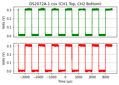
[12]:
ch = w.channels[0]
plt.subplot(211)
plt.plot(ch.times*1e6, ch.volts, color='green')
plt.title(filename + " (CH1 Top, CH2 Bottom)")
plt.ylabel("Volts (V)")
plt.grid(True)
plt.xticks([])

ch = w.channels[1]
plt.subplot(212)
plt.plot(ch.times*1e6, ch.volts, color='red')
plt.xlabel("Time (µs)")
plt.ylabel("Volts (V)")
plt.grid(True)

plt.show()
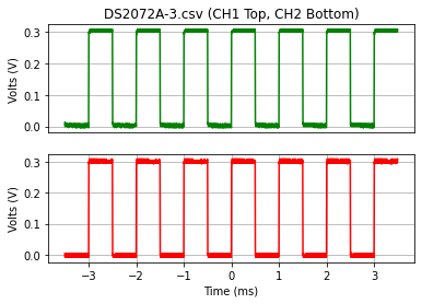
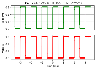
DS2072A-3

First the .csv data
Let’s look at what the accompanying .csv data looks like.
[13]:
filename = "DS2072A-3.csv"
csv_data = read_rigol_csv(repo+filename)

plt.subplot(211)
plt.plot(csv_data[0]*1e3,csv_data[1], color='green')
plt.title(filename + " (CH1 Top, CH2 Bottom)")
plt.ylabel("Volts (V)")
#plt.ylim(-10,10)
plt.grid(True)
plt.xticks([])

plt.subplot(212)
plt.plot(csv_data[0]*1e3,csv_data[2], color='red')
plt.xlabel("Time (ms)")
plt.ylabel("Volts (V)")
plt.grid(True)
#plt.ylim(-2,2)

plt.show()
Now for the wfm data
First let’s have look at the description of the internal file structure. We see that only channel 1 has been enabled.
[14]:
# raw=true is needed because this is a binary file
wfm_url = repo + "DS2072A-3.wfm" + "?raw=true"

w = rigol.Wfm.from_url(wfm_url, 'DS2000')
description = w.describe()
print(description)
downloading 'https://github.com/scottprahl/RigolWFM/raw/master/wfm/DS2072A-3.wfm?raw=true'
    General:
        File Model   = wfm2000
        User Model   = DS2000
        Parser Model = wfm2000
        Firmware     = 00.03.05.03.03
        Filename     = DS2072A-3.wfm
        Channels     = [1, 2]

     Channel 1:
         Coupling =       DC
            Scale =   100.00 mV/div
           Offset =    60.00 mV
            Probe =    0.01X
         Inverted =    False

        Time Base =  500.000 µs/div
           Offset =    0.000  s
            Delta =    1.000 ns/point
           Points =  7000000

         Count    = [        1,        2,        3  ...   6999999,  7000000]
           Raw    = [      218,      218,      218  ...       218,      218]
           Times  = [-3.500 ms,-3.500 ms,-3.500 ms  ...  3.500 ms, 3.500 ms]
           Volts  = [304.00 mV,304.00 mV,304.00 mV  ... 304.00 mV,304.00 mV]

     Channel 2:
         Coupling =       DC
            Scale =   100.00 mV/div
           Offset =  -302.00 mV
            Probe =    0.01X
         Inverted =    False

        Time Base =  500.000 µs/div
           Offset =    0.000  s
            Delta =    1.000 ns/point
           Points =  7000000

         Count    = [        1,        2,        3  ...   6999999,  7000000]
           Raw    = [      127,      126,      128  ...       127,      127]
           Times  = [-3.500 ms,-3.500 ms,-3.500 ms  ...  3.500 ms, 3.500 ms]
           Volts  = [302.00 mV,298.00 mV,306.00 mV  ... 302.00 mV,302.00 mV]
[15]:
ch = w.channels[0]
plt.subplot(211)
plt.plot(ch.times*1e3, ch.volts, color='green')
plt.title(filename + " (CH1 Top, CH2 Bottom)")
plt.ylabel("Volts (V)")
#plt.ylim(-10,10)
plt.grid(True)
plt.xticks([])

ch = w.channels[1]
plt.subplot(212)
plt.plot(ch.times*1e3, ch.volts, color='red')
plt.xlabel("Time (ms)")
plt.ylabel("Volts (V)")
#plt.ylim(-2,2)
plt.grid(True)

plt.show()
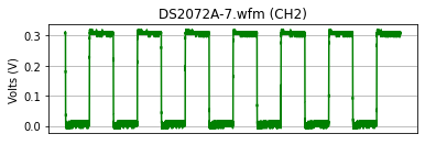
DS2072A-7

[16]:
filename = "DS2072A-7.wfm"
repo = "../wfm"
w = rigol.Wfm.from_file(f"{repo}/{filename}", 'DS2072A')
description = w.describe()
print(description)
    General:
        File Model   = wfm2000
        User Model   = DS2072A
        Parser Model = wfm2000
        Firmware     = 00.03.05.03.03
        Filename     = DS2072A-7.wfm
        Channels     = [2]

     Channel 2:
         Coupling =       DC
            Scale =   200.00 mV/div
           Offset =  -192.00 mV
            Probe =    0.01X
         Inverted =    False

        Time Base =  500.000 µs/div
           Offset =    0.000  s
            Delta =    1.000 ns/point
           Points =  7000000

         Count    = [        1,        2,        3  ...   6999999,  7000000]
           Raw    = [      142,      142,      142  ...       141,      142]
           Times  = [-3.500 ms,-3.500 ms,-3.500 ms  ...  3.500 ms, 3.500 ms]
           Volts  = [312.00 mV,312.00 mV,312.00 mV  ... 304.00 mV,312.00 mV]
[17]:
ch = w.channels[0]
plt.subplot(211)
plt.plot(ch.times*1e3, ch.volts, color='green')
plt.title(f"{filename} (CH2)")
plt.ylabel("Volts (V)")
plt.grid(True)
plt.xticks([])

plt.show()
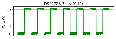
[18]:
filename = "DS2072A-7.csv"
csv_data = read_rigol_csv(f"{repo}/{filename}")

plt.subplot(211)
plt.plot(csv_data[0]*1e3,csv_data[1], color='green')
plt.title(filename + " (CH2)")
plt.ylabel("Volts (V)")
#plt.ylim(-10,10)
plt.grid(True)
plt.xticks([])


plt.show()
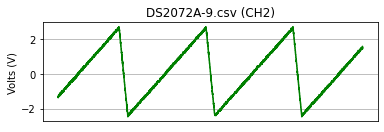
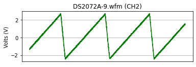
DS2072A-9

Test for large memory bank if CH1 is unselected.
[19]:
filename = "DS2072A-9.wfm"
repo = "../wfm"
w = rigol.Wfm.from_file(f"{repo}/{filename}", 'DS2072A')
description = w.describe()
print(description)
    General:
        File Model   = wfm2000
        User Model   = DS2072A
        Parser Model = wfm2000
        Firmware     = 00.03.06.00.00
        Filename     = DS2072A-9.wfm
        Channels     = [2]

     Channel 2:
         Coupling =       DC
            Scale =     2.00  V/div
           Offset =     0.00  V
            Probe =    0.01X
         Inverted =    False

        Time Base =  500.000 µs/div
           Offset =    0.000  s
            Delta =  500.000 ns/point
           Points =    14000

         Count    = [        1,        2,        3  ...     13999,    14000]
           Raw    = [      110,      111,      111  ...       146,      146]
           Times  = [-3.500 ms,-3.499 ms,-3.499 ms  ...  3.499 ms, 3.500 ms]
           Volts  = [ -1.36  V, -1.28  V, -1.28  V  ...   1.52  V,  1.52  V]
[20]:
ch = w.channels[0]
plt.subplot(211)
plt.plot(ch.times*1e3, ch.volts, color='green')
plt.title(f"{filename} (CH2)")
plt.ylabel("Volts (V)")
plt.grid(True)
plt.xticks([])

plt.show()
[21]:
filename = "DS2072A-9.csv"
csv_data = read_rigol_csv(f"{repo}/{filename}")

plt.subplot(211)
plt.plot(csv_data[0]*1e3,csv_data[1], color='green')
plt.title(filename + " (CH2)")
plt.ylabel("Volts (V)")
#plt.ylim(-10,10)
plt.grid(True)
plt.xticks([])


plt.show()