Agilent and Keysight Binary Waveform Examples
Scott Prahl
Mar 2026
[1]:
%config InlineBackend.figure_format = 'retina'

import io

import numpy as np
import matplotlib.pyplot as plt
import requests
from RigolWFM import Wfm

repo = "https://raw.githubusercontent.com/scottprahl/RigolWFM/main/tests/files/"


def sample_url(relative_path: str) -> str:
    return repo + relative_path


def _time_scale(times):
    span = float(abs(times[-1] - times[0])) if len(times) > 1 else 1.0
    if span >= 1e-3:
        return 1e3, "ms"
    if span >= 1e-6:
        return 1e6, "us"
    if span >= 1e-9:
        return 1e9, "ns"
    return 1e12, "ps"


def _volt_scale(values):
    peak = max(float(np.max(np.abs(v))) for v in values) if values else 1.0
    if peak >= 1.0:
        return 1.0, "V"
    if peak >= 1e-3:
        return 1e3, "mV"
    if peak >= 1e-6:
        return 1e6, "uV"
    return 1e9, "nV"


def plot_analog_channels(w, title=None, max_points=5000):
    active = [ch for ch in w.channels if ch.times is not None and ch.volts is not None]
    if not active:
        print("No analog channels are enabled in this capture.")
        return

    colors = ["green", "red", "blue", "orange"]
    t_scale, t_unit = _time_scale(active[0].times)
    v_scale, v_unit = _volt_scale([ch.volts for ch in active])

    fig, axes = plt.subplots(len(active), 1, sharex=True, figsize=(10, 2.5 * len(active)))
    if len(active) == 1:
        axes = [axes]

    for ax, ch, color in zip(axes, active, colors):
        stride = max(len(ch.times) // max_points, 1)
        ax.plot(ch.times[::stride] * t_scale, ch.volts[::stride] * v_scale, color=color)
        ax.set_ylabel(v_unit)
        ax.set_title(f"CH{ch.channel_number}  {ch.points} points")
        ax.grid(True)

    axes[-1].set_xlabel(f"Time ({t_unit})")
    if title:
        fig.suptitle(title)
    plt.tight_layout()
    plt.show()


def plot_logic_window(w, names=None, start=0, stop=4000, title=None):
    if not w.logic_channels:
        print("No logic channels are enabled in this capture.")
        return

    if names is None:
        names = list(w.logic_channels)

    if w.logic_times is None:
        times = np.arange(len(next(iter(w.logic_channels.values()))), dtype=np.float64)
    else:
        times = w.logic_times

    stop = min(stop, len(times))
    t_scale, t_unit = _time_scale(times[start:stop])

    fig, axes = plt.subplots(len(names), 1, sharex=True, figsize=(10, 1.6 * len(names)))
    if len(names) == 1:
        axes = [axes]

    colors = ["green", "red", "blue", "orange", "purple", "brown"]
    for ax, name, color in zip(axes, names, colors):
        trace = w.logic_channels[name]
        ax.step(times[start:stop] * t_scale, trace[start:stop], where="post", color=color)
        ax.set_ylim(-0.2, 1.2)
        ax.set_yticks([0, 1])
        ax.set_ylabel(name)
        ax.grid(True)

    axes[-1].set_xlabel(f"Time ({t_unit})")
    if title:
        fig.suptitle(title)
    plt.tight_layout()
    plt.show()
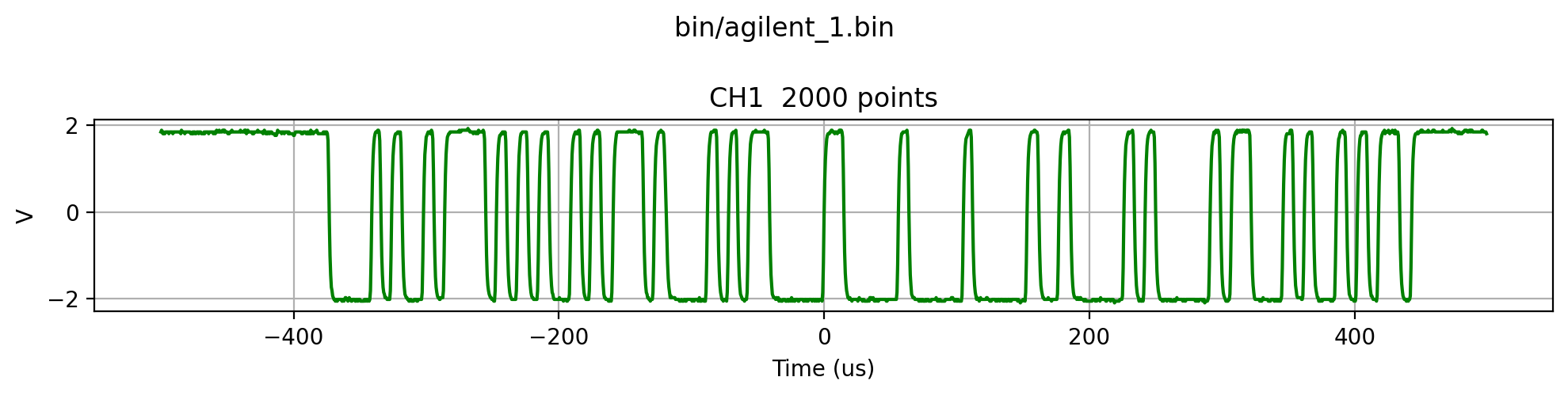
agilent_1.bin - Single-channel analog capture
Oscilloscope screenshot
[2]:
filename = "bin/agilent_1.bin"
w = Wfm.from_url(sample_url(filename), "Keysight")
print(w.describe())
    General:
        File Model   = DSO-X 1102G
        Serial Number = CN00000000
        User Model   = Keysight
        Parser Model = agilent_bin
        Firmware     = unknown
        Filename     = agilent_1.bin
        Channels     = [1]

    Trigger:
        Derived Level (CH1) = -80.40 mV

     Channel 1:
         Coupling =  unknown
            Scale =   502.51 mV/div
           Offset =     0.00  V
            Probe =       1X
         Inverted =    False

        Time Base =  100.000 µs/div
           Offset =    0.000  s
            Delta =  500.000 ns/point
           Points =     2000

         Count    = [        1,        2,        3  ...      1999,     2000]
           Raw    = [        5,        3,        5  ...         5,        8]
           Times  = [-500.063 µs,-499.563 µs,-499.063 µs  ... 498.937 µs,499.437 µs]
           Volts  = [  1.85  V,  1.89  V,  1.85  V  ...   1.85  V,  1.81  V]
downloading 'https://raw.githubusercontent.com/scottprahl/RigolWFM/main/tests/files/bin/agilent_1.bin'
Plot the decoded channel
[3]:
plot_analog_channels(w, title=filename)
agilent_3.bin - Two-channel capture
Oscilloscope screenshot
[4]:
filename = "bin/agilent_3.bin"
w = Wfm.from_url(sample_url(filename), "Keysight")
print(w.describe())
    General:
        File Model   = DSO-X 1102G
        Serial Number = CN00000000
        User Model   = Keysight
        Parser Model = agilent_bin
        Firmware     = unknown
        Filename     = agilent_3.bin
        Channels     = [1, 2]

    Trigger:
        Derived Level (CH1) = 180.90 mV
        Derived Level (CH2) = -1.22  V

     Channel 1:
         Coupling =  unknown
            Scale =   703.52 mV/div
           Offset =     0.00  V
            Probe =       1X
         Inverted =    False

        Time Base =  200.000 ns/div
           Offset =    0.000  s
            Delta =  500.000 ps/point
           Points =     4000

         Count    = [        1,        2,        3  ...      3999,     4000]
           Raw    = [      116,      116,      116  ...       116,      116]
           Times  = [-1.000 µs,-999.500 ns,-999.000 ns  ... 999.000 ns,999.500 ns]
           Volts  = [180.90 mV,180.90 mV,180.90 mV  ... 180.90 mV,180.90 mV]

     Channel 2:
         Coupling =  unknown
            Scale =   402.01 mV/div
           Offset =     0.00  V
            Probe =       1X
         Inverted =    False

        Time Base =  200.000 ns/div
           Offset =    0.000  s
            Delta =  500.000 ps/point
           Points =     4000

         Count    = [        1,        2,        3  ...      3999,     4000]
           Raw    = [        6,        6,        6  ...       251,      251]
           Times  = [-1.000 µs,-999.500 ns,-999.000 ns  ... 999.000 ns,999.500 ns]
           Volts  = [  1.52  V,  1.52  V,  1.52  V  ...  -1.58  V, -1.58  V]
downloading 'https://raw.githubusercontent.com/scottprahl/RigolWFM/main/tests/files/bin/agilent_3.bin'
Plot both enabled channels
[5]:
plot_analog_channels(w, title=filename)

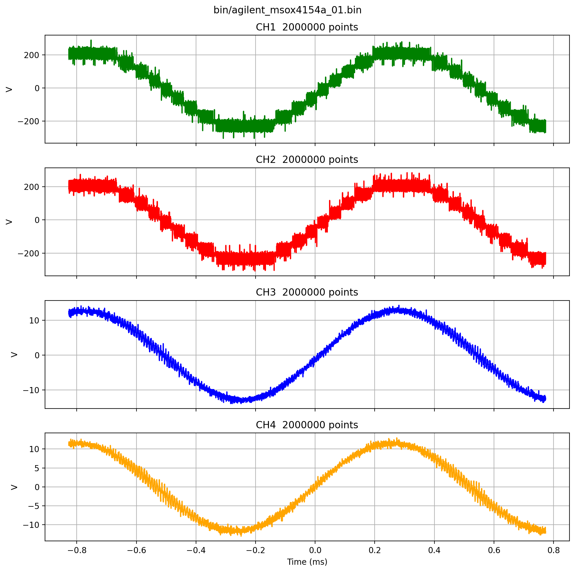
agilent_msox4154a_01.bin - Four-channel MSO-X capture
This file is much larger than the small demo fixtures, so the plot below is decimated for readability.
[6]:
filename = "bin/agilent_msox4154a_01.bin"
w = Wfm.from_url(sample_url(filename), "Keysight")
print(w.describe())
downloading 'https://raw.githubusercontent.com/scottprahl/RigolWFM/main/tests/files/bin/agilent_msox4154a_01.bin'
    General:
        File Model   = MSO-X 4154A
        Serial Number = MY00000000
        User Model   = Keysight
        Parser Model = agilent_bin
        Firmware     = unknown
        Filename     = agilent_msox4154a_01.bin
        Channels     = [1, 2, 3, 4]

    Trigger:
        Derived Level (CH1) = -57.75  V
        Derived Level (CH2) = 13.39  V
        Derived Level (CH3) = -901.82 mV
        Derived Level (CH4) = 377.09 mV

     Channel 1:
         Coupling =  unknown
            Scale =    78.24  V/div
           Offset =     0.00  V
            Probe =       1X
         Inverted =    False

        Time Base =  200.000 µs/div
           Offset =    0.000  s
            Delta =  800.000 ps/point
           Points =  2000000

         Count    = [        1,        2,        3  ...   1999999,  2000000]
           Raw    = [       26,       24,       24  ...       225,      227]
           Times  = [-826.613 µs,-826.612 µs,-826.611 µs  ... 773.386 µs,773.386 µs]
           Volts  = [233.46  V,236.81  V,236.81  V  ... -258.59  V,-261.94  V]

     Channel 2:
         Coupling =  unknown
            Scale =    79.50  V/div
           Offset =     0.00  V
            Probe =       1X
         Inverted =    False

        Time Base =  200.000 µs/div
           Offset =    0.000  s
            Delta =  800.000 ps/point
           Points =  2000000

         Count    = [        1,        2,        3  ...   1999999,  2000000]
           Raw    = [       47,       47,       45  ...       201,      201]
           Times  = [-826.613 µs,-826.612 µs,-826.611 µs  ... 773.386 µs,773.386 µs]
           Volts  = [187.45  V,187.45  V,190.79  V  ... -197.49  V,-197.49  V]

     Channel 3:
         Coupling =  unknown
            Scale =     3.79  V/div
           Offset =     0.00  V
            Probe =       1X
         Inverted =    False

        Time Base =  200.000 µs/div
           Offset =    0.000  s
            Delta =  800.000 ps/point
           Points =  2000000

         Count    = [        1,        2,        3  ...   1999999,  2000000]
           Raw    = [       22,       21,       25  ...       232,      232]
           Times  = [-826.613 µs,-826.612 µs,-826.611 µs  ... 773.386 µs,773.386 µs]
           Volts  = [ 12.49  V, 12.65  V, 12.15  V  ... -12.45  V,-12.45  V]

     Channel 4:
         Coupling =  unknown
            Scale =     3.39  V/div
           Offset =     0.00  V
            Probe =       1X
         Inverted =    False

        Time Base =  200.000 µs/div
           Offset =    0.000  s
            Delta =  800.000 ps/point
           Points =  2000000

         Count    = [        1,        2,        3  ...   1999999,  2000000]
           Raw    = [       20,       22,       22  ...       238,      241]
           Times  = [-826.613 µs,-826.612 µs,-826.611 µs  ... 773.386 µs,773.386 µs]
           Volts  = [ 11.26  V, 11.09  V, 11.09  V  ... -12.01  V,-12.34  V]
Plot all four channels
[7]:
plot_analog_channels(w, title=filename, max_points=8000)