Rigol DHO1000 Waveform Examples
Scott Prahl
Mar 2026
[1]:
%config InlineBackend.figure_format = 'retina'

import numpy as np
import matplotlib.pyplot as plt
import imageio.v3 as iio

from RigolWFM import Wfm, DHO1000_scopes

repo = "https://raw.githubusercontent.com/scottprahl/RigolWFM/main/tests/files/"
A list of Rigol scopes in the DHO1000 family is:
[2]:
print(DHO1000_scopes)
['DHO', 'DHO800', 'DHO1000', 'DHO804', 'DHO812', 'DHO814', 'DHO824', 'DHO1072', 'DHO1074', 'DHO1102', 'DHO1202', 'DHO1204']
DHO1074 - Single-channel .wfm capture
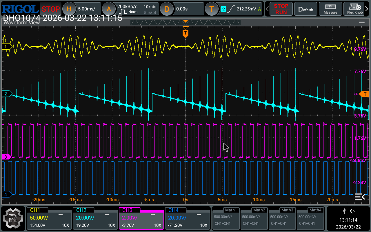
Look at a screen shot
This capture was taken on a DHO1074 oscilloscope with CH1 active, measuring a 3.3 V logic signal.
Import the .wfm data
[3]:
filename = "wfm/DHO1074.wfm"

w = Wfm.from_url(repo + filename, "DHO")
downloading 'https://raw.githubusercontent.com/scottprahl/RigolWFM/main/tests/files/wfm/DHO1074.wfm'
Textual description of the waveform
[4]:
description = w.describe()
print(description)
    General:
        File Model   = DHO1000
        User Model   = DHO
        Parser Model = dho1000
        Firmware     = unknown
        Filename     = DHO1074.wfm
        Channels     = [1, 2, 3, 4]

    Trigger:
        Derived Level (CH1) = -919.98 mV
        Derived Level (CH2) = -3.34  V
        Derived Level (CH3) = 2.95  V
        Derived Level (CH4) = 29.00  V

     Channel 1:
         Coupling =  unknown
            Scale =    54.61  V/div
           Offset =   154.00  V
            Probe =       1X
         Inverted =    False

        Time Base =    5.000 ms/div
           Offset =    0.000  s
            Delta =    5.000 µs/point
           Points =    10000

         Count    = [        1,        2,        3  ...      9999,    10000]
           Raw    = [      207,      207,      208  ...       207,      207]
           Times  = [-25.000 ms,-24.995 ms,-24.990 ms  ... 24.990 ms,24.995 ms]
           Volts  = [-17.81  V,-18.49  V,-16.47  V  ... -18.59  V,-18.93  V]

     Channel 2:
         Coupling =  unknown
            Scale =    21.85  V/div
           Offset =    19.20  V
            Probe =       1X
         Inverted =    False

        Time Base =    5.000 ms/div
           Offset =    0.000  s
            Delta =    5.000 µs/point
           Points =    10000

         Count    = [        1,        2,        3  ...      9999,    10000]
           Raw    = [      144,      169,      188  ...       121,      126]
           Times  = [-25.000 ms,-24.995 ms,-24.990 ms  ... 24.990 ms,24.995 ms]
           Volts  = [ -7.67  V,  9.22  V, 22.23  V  ... -23.44  V,-20.46  V]

     Channel 3:
         Coupling =  unknown
            Scale =     2.18  V/div
           Offset =    -3.76  V
            Probe =       1X
         Inverted =    False

        Time Base =    5.000 ms/div
           Offset =    0.000  s
            Delta =    5.000 µs/point
           Points =    10000

         Count    = [        1,        2,        3  ...      9999,    10000]
           Raw    = [      115,      116,      115  ...       116,      116]
           Times  = [-25.000 ms,-24.995 ms,-24.990 ms  ... 24.990 ms,24.995 ms]
           Volts  = [  2.90  V,  2.94  V,  2.91  V  ...   2.95  V,  2.96  V]

     Channel 4:
         Coupling =  unknown
            Scale =    21.85  V/div
           Offset =   -71.20  V
            Probe =       1X
         Inverted =    False

        Time Base =    5.000 ms/div
           Offset =    0.000  s
            Delta =    5.000 µs/point
           Points =    10000

         Count    = [        1,        2,        3  ...      9999,    10000]
           Raw    = [       66,       66,       66  ...        66,       66]
           Times  = [-25.000 ms,-24.995 ms,-24.990 ms  ... 24.990 ms,24.995 ms]
           Volts  = [ 29.46  V, 29.18  V, 29.27  V  ...  29.32  V, 29.23  V]
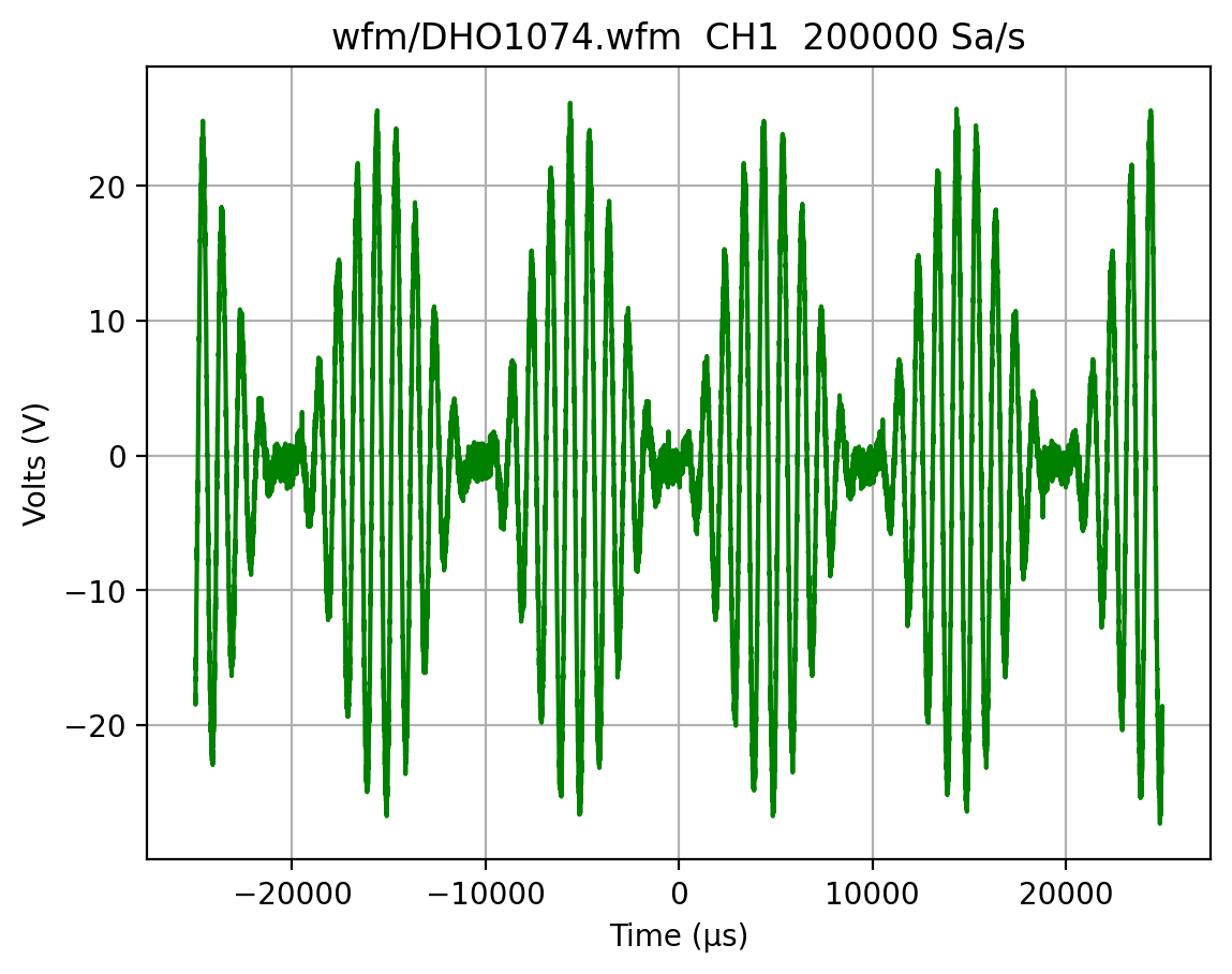
Plot the waveform
[5]:
ch = w.channels[0]

plt.plot(ch.times * 1e6, ch.volts, color="green")
plt.title("%s  CH%d  %.0f Sa/s" % (filename, ch.channel_number, 1 / ch.seconds_per_point))
plt.xlabel("Time (µs)")
plt.ylabel("Volts (V)")
plt.grid(True)

plt.show()
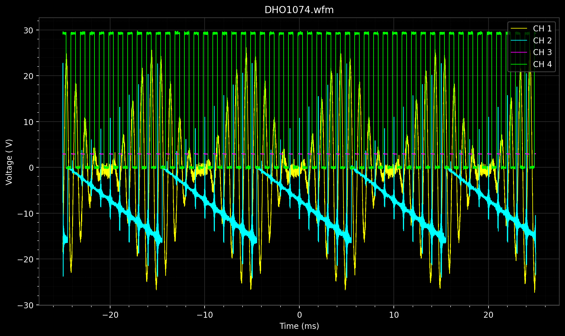
The w.plot() convenience method draws all enabled channels automatically:
[6]:
w.plot()
plt.show()
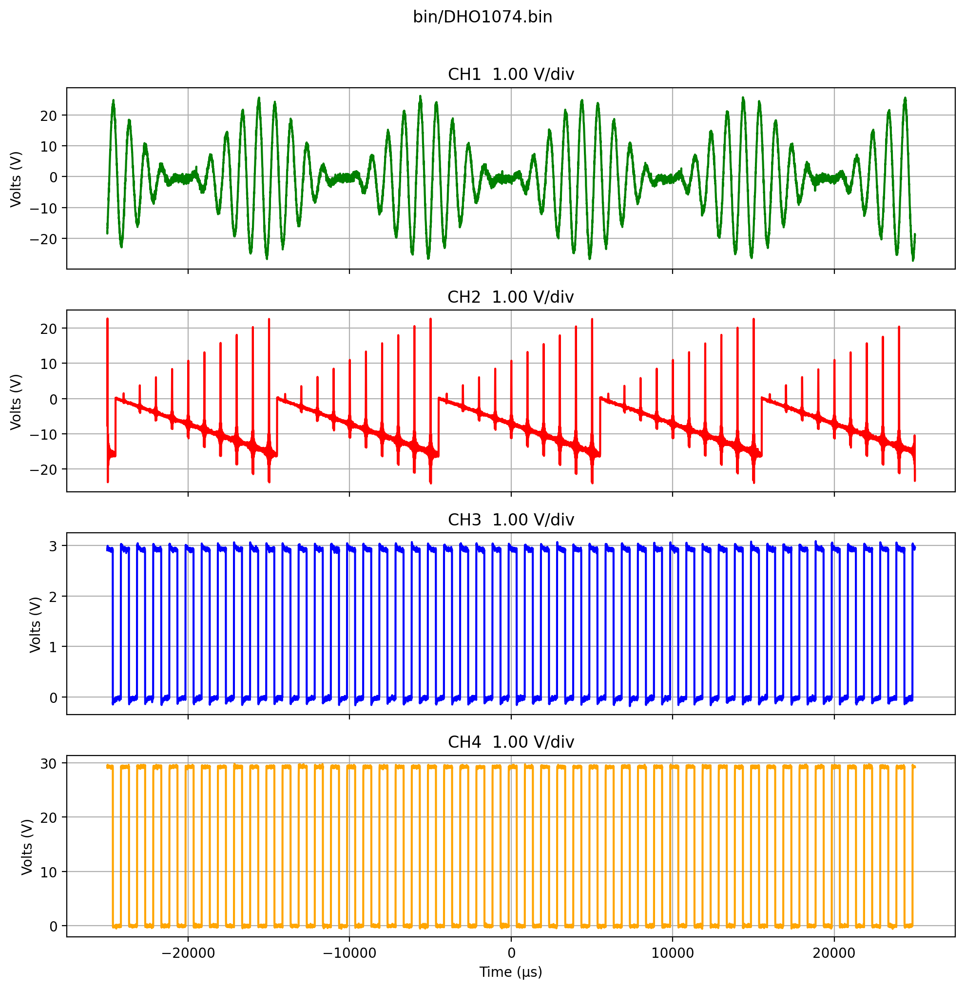
DHO1074 - Four-channel .bin capture
Look at a screen shot
This capture was taken on a DHO1074 oscilloscope with all four channels enabled. The .bin format is documented in the DHO1000 User Guide, Section 19.2.4. It stores calibrated float32 voltage values directly - no additional scaling is required.
Import the .bin data
[7]:
filename = "bin/DHO1074.bin"
w = Wfm.from_url(repo + filename)
downloading 'https://raw.githubusercontent.com/scottprahl/RigolWFM/main/tests/files/bin/DHO1074.bin'
Textual description of the waveform
[8]:
description = w.describe()
print(description)
    General:
        File Model   = DHO1000 (BIN)
        User Model   = auto
        Parser Model = dho1000
        Firmware     = unknown
        Filename     = DHO1074.bin
        Channels     = [1, 2, 3, 4]

    Trigger:
        Derived Level (CH1) = -913.33 mV
        Derived Level (CH2) = -3.34  V
        Derived Level (CH3) = 2.95  V
        Derived Level (CH4) = 28.99  V

     Channel 1:
         Coupling =  unknown
            Scale =     1.00  V/div
           Offset =     0.00  V
            Probe =       1X
         Inverted =    False

        Time Base =    5.000 ms/div
           Offset =    0.000  s
            Delta =    5.000 µs/point
           Points =    10000

         Count    = [        1,        2,        3  ...      9999,    10000]
           Raw    = [       58,       55,       63  ...        55,       54]
           Times  = [-25.000 ms,-24.995 ms,-24.990 ms  ... 24.990 ms,24.995 ms]
           Volts  = [-17.81  V,-18.48  V,-16.47  V  ... -18.59  V,-18.93  V]

     Channel 2:
         Coupling =  unknown
            Scale =     1.00  V/div
           Offset =     0.00  V
            Probe =       1X
         Inverted =    False

        Time Base =    5.000 ms/div
           Offset =    0.000  s
            Delta =    5.000 µs/point
           Points =    10000

         Count    = [        1,        2,        3  ...      9999,    10000]
           Raw    = [       98,      164,      214  ...        36,       48]
           Times  = [-25.000 ms,-24.995 ms,-24.990 ms  ... 24.990 ms,24.995 ms]
           Volts  = [ -7.67  V,  9.22  V, 22.23  V  ... -23.44  V,-20.46  V]

     Channel 3:
         Coupling =  unknown
            Scale =     1.00  V/div
           Offset =     0.00  V
            Probe =       1X
         Inverted =    False

        Time Base =    5.000 ms/div
           Offset =    0.000  s
            Delta =    5.000 µs/point
           Points =    10000

         Count    = [        1,        2,        3  ...      9999,    10000]
           Raw    = [      139,      139,      139  ...       139,      139]
           Times  = [-25.000 ms,-24.995 ms,-24.990 ms  ... 24.990 ms,24.995 ms]
           Volts  = [  2.90  V,  2.94  V,  2.91  V  ...   2.95  V,  2.96  V]

     Channel 4:
         Coupling =  unknown
            Scale =     1.00  V/div
           Offset =     0.00  V
            Probe =       1X
         Inverted =    False

        Time Base =    5.000 ms/div
           Offset =    0.000  s
            Delta =    5.000 µs/point
           Points =    10000

         Count    = [        1,        2,        3  ...      9999,    10000]
           Raw    = [      243,      241,      242  ...       242,      242]
           Times  = [-25.000 ms,-24.995 ms,-24.990 ms  ... 24.990 ms,24.995 ms]
           Volts  = [ 29.46  V, 29.18  V, 29.27  V  ...  29.32  V, 29.23  V]
Plot all four channels
The .bin format stores each channel independently. All four are plotted below.
[9]:
colors = ["green", "red", "blue", "orange"]
active = [ch for ch in w.channels if ch.volts is not None]
n = len(active)

fig, axes = plt.subplots(n, 1, sharex=True, figsize=(10, 2.5 * n))
if n == 1:
    axes = [axes]

for ax, ch, color in zip(axes, active, colors):
    ax.plot(ch.times * 1e6, ch.volts, color=color)
    ax.set_ylabel("Volts (V)")
    ax.set_title("CH%d  %.2f V/div" % (ch.channel_number, ch.volt_per_division))
    ax.grid(True)

axes[-1].set_xlabel("Time (µs)")
fig.suptitle(filename, y=1.01)
plt.tight_layout()
plt.show()
The w.plot() convenience method draws the same result in a single call:
[10]:
w.plot()
plt.show()

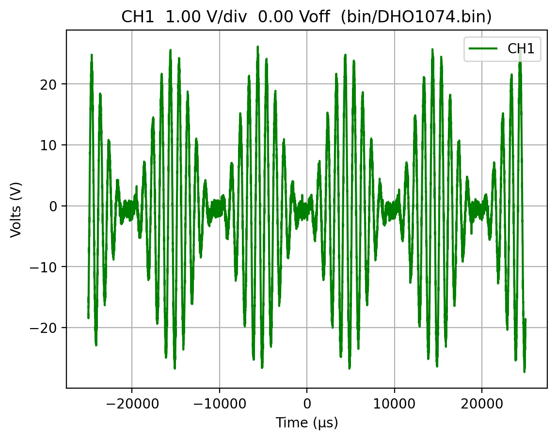
Select a single channel from a multi-channel .bin file
Pass the selected argument to Wfm.from_file() to load only specific channels. This avoids allocating memory for channels you do not need.
[11]:
filename = "bin/DHO1074.bin"
w1 = Wfm.from_url(repo + filename, selected="1")

ch = w1.channels[0]
plt.title("CH%d  %.2f V/div  %.2f Voff  (%s)" % (ch.channel_number, ch.volt_per_division, ch.volt_offset, filename))
plt.plot(ch.times * 1e6, ch.volts, color="green", label="CH1")
plt.xlabel("Time (µs)")
plt.ylabel("Volts (V)")
plt.legend(loc="upper right")
plt.grid(True)
plt.show()
downloading 'https://raw.githubusercontent.com/scottprahl/RigolWFM/main/tests/files/bin/DHO1074.bin'
Format comparison: .wfm vs .bin
DHO1074.wfm and DHO1074.bin are captures from the same oscilloscope model (DHO1074)
but from different measurement sessions, so a direct sample-by-sample comparison is
not meaningful here. The table below summarises the key differences between the two formats.
Property |
|
|
|---|---|---|
Documented |
Yes (User Guide §19.2.4) |
No (reverse-engineered) |
Sample type |
float32 (calibrated V) |
uint16 (raw ADC) |
Channels |
All enabled, separate |
CH1 only in tested files |
Metadata |
In waveform headers |
zlib-compressed blocks |
x_origin sign |
Positive (negate for t0) |
Negative (use directly) |
[12]:
wfm = Wfm.from_url(repo + "wfm/DHO1074.wfm", "DHO")

wfm_ch = wfm.channels[0]


print("DHO1074.wfm")

print("  Points     : %d" % len(wfm_ch.times))

print("  Delta t    : %.3f µs" % (wfm_ch.seconds_per_point * 1e6))

print("  Time span  : %.3f ms" % ((wfm_ch.times[-1] - wfm_ch.times[0]) * 1e3))

print("  Vmin / Vmax: %.3f V / %.3f V" % (wfm_ch.volts.min(), wfm_ch.volts.max()))

print()


bin_ = Wfm.from_url(repo + "bin/DHO1074.bin", selected="1")

bin_ch = bin_.channels[0]


print("DHO1074.bin  (CH1 only)")

print("  Points     : %d" % len(bin_ch.times))

print("  Delta t    : %.3f µs" % (bin_ch.seconds_per_point * 1e6))

print("  Time span  : %.3f ms" % ((bin_ch.times[-1] - bin_ch.times[0]) * 1e3))

print("  Vmin / Vmax: %.3f V / %.3f V" % (bin_ch.volts.min(), bin_ch.volts.max()))
downloading 'https://raw.githubusercontent.com/scottprahl/RigolWFM/main/tests/files/wfm/DHO1074.wfm'
DHO1074.wfm
  Points     : 10000
  Delta t    : 5.000 µs
  Time span  : 49.995 ms
  Vmin / Vmax: -27.320 V / 26.153 V

DHO1074.bin  (CH1 only)
  Points     : 10000
  Delta t    : 5.000 µs
  Time span  : 49.995 ms
  Vmin / Vmax: -27.313 V / 26.160 V
downloading 'https://raw.githubusercontent.com/scottprahl/RigolWFM/main/tests/files/bin/DHO1074.bin'
[ ]: