Rigol DS1000E Waveform Examples
Scott Prahl
Mar 2026
[1]:
%config InlineBackend.figure_format = 'retina'

import numpy as np
import matplotlib.pyplot as plt
import imageio.v3 as iio

from RigolWFM import Wfm, DS1000E_scopes

repo = "https://raw.githubusercontent.com/scottprahl/RigolWFM/main/tests/files/"
Introduction
This notebook illustrates shows how to extract signals from a .wfm file created by a the Rigol DS1000E scope. It also validates that the process works by comparing with .csv and screenshots.
Two different .wfm files are examined one for the DS1052E scope and one for the DS1102E scope. The accompanying .csv files seem to have t=0 in the zero in the center of the waveform.
The list of Rigol scopes that should produce the same file format are:
[2]:
print(DS1000E_scopes[:])
['E', '1000E', 'DS1000E', 'DS1102E', 'DS1052E']
DS1052E
.wfm file from a Rigol DS1052E scope. This test file accompanies wfm_view.exe a freeware program from http://www.hakasoft.com.au.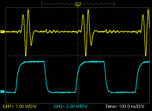
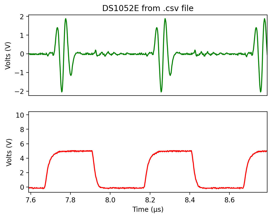
Now let’s look at plot of the data from the corresponding .csv file created by wfm_view.exe
[3]:
csv_filename_52 = repo + "wfm/DS1052E.csv"

csv_data = np.genfromtxt(csv_filename_52, delimiter=",", skip_header=19, skip_footer=2, encoding="latin1").T

center_time = csv_data[0][-1] * 1e6 / 2

plt.subplot(211)
plt.plot(csv_data[0] * 1e6, csv_data[1], color="green")
plt.title("DS1052E from .csv file")
plt.ylabel("Volts (V)")
plt.xlim(center_time - 0.6, center_time + 0.6)
plt.xticks([])

plt.subplot(212)
plt.plot(csv_data[0] * 1e6, csv_data[2], color="red")
plt.xlabel("Time (µs)")
plt.ylabel("Volts (V)")
plt.xlim(center_time - 0.6, center_time + 0.6)

plt.show()
Now for the .wfm data
First a textual description.
[4]:
wfm_url = repo + "wfm/DS1052E.wfm?raw=true"
w = Wfm.from_url(wfm_url, "1000E")
description = w.describe()
print(description)
    General:
        File Model   = DS1000E
        User Model   = 1000E
        Parser Model = wfm1000e
        Firmware     = unknown
        Filename     = DS1052E.wfm
        Channels     = [1, 2]

    Trigger:
        Mode     = edge
        Source   = CH2
        Level    = 2.40  V
        Sweep    = AUTO
        Coupling = DC
        Derived Level     = 3.84  V

     Channel 1:
         Coupling =  unknown
            Scale =     1.00  V/div
           Offset =     2.00  V
            Probe =      10X
         Inverted =    False

        Time Base =  100.000 ns/div
           Offset =    0.000  s
            Delta =    2.000 ns/point
           Points =     8192

         Count    = [        1,        2,        3  ...      8191,     8192]
           Raw    = [       76,       76,       76  ...        76,       76]
           Times  = [-8.192 µs,-8.190 µs,-8.188 µs  ...  8.188 µs, 8.190 µs]
           Volts  = [-40.00 mV,-40.00 mV,-40.00 mV  ... -40.00 mV,-40.00 mV]

     Channel 2:
         Coupling =  unknown
            Scale =     2.00  V/div
           Offset =    -6.00  V
            Probe =       1X
         Inverted =    False

        Time Base =  100.000 ns/div
           Offset =    0.000  s
            Delta =    2.000 ns/point
           Points =     8192

         Count    = [        1,        2,        3  ...      8191,     8192]
           Raw    = [      203,      203,      203  ...       138,      138]
           Times  = [-8.192 µs,-8.190 µs,-8.188 µs  ...  8.188 µs, 8.190 µs]
           Volts  = [-240.00 mV,-240.00 mV,-240.00 mV  ...   4.96  V,  4.96  V]
downloading 'https://raw.githubusercontent.com/scottprahl/RigolWFM/main/tests/files/wfm/DS1052E.wfm?raw=true'
[5]:
ch = w.channels[0]
plt.subplot(211)
plt.plot(ch.times * 1e6, ch.volts, color="green")
plt.title("DS1052E from .wfm file")
plt.ylabel("Volts (V)")
plt.xlim(-0.6, 0.6)

plt.xticks([])

ch = w.channels[1]
plt.subplot(212)
plt.plot(ch.times * 1e6, ch.volts, color="red")
plt.xlabel("Time (ms)")
plt.ylabel("Volts (V)")
plt.xlim(-0.6, 0.6)

plt.show()

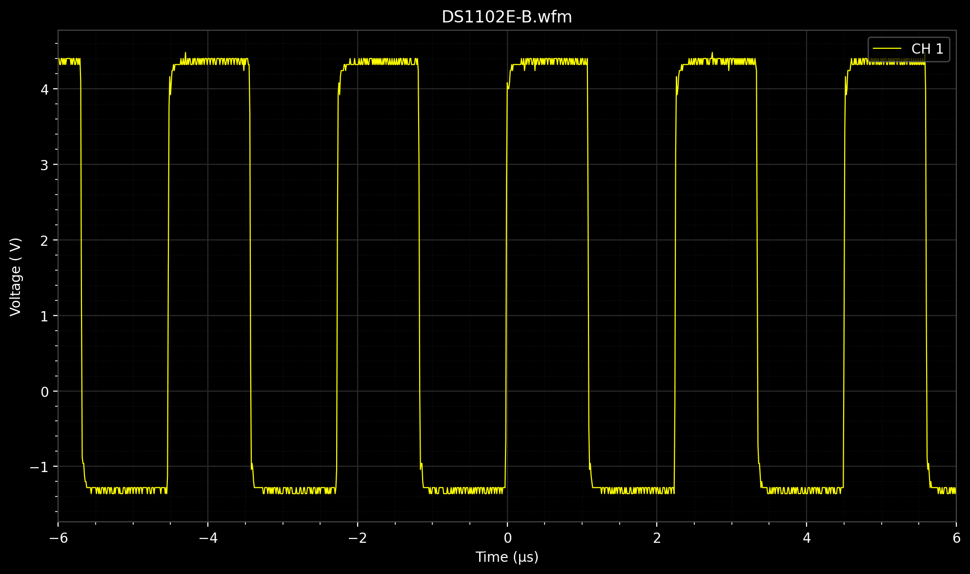
DS1102E-B
First the .csv data
This file only has one active channel. Let’s look at what the accompanying .csv data looks like.
[6]:
csv_filename = repo + "wfm/DS1102E-B.csv"

my_data = np.genfromtxt(csv_filename, delimiter=",", skip_header=2).T

plt.plot(my_data[0] * 1e6, my_data[1])
plt.xlabel("Time (µs)")
plt.ylabel("Volts (V)")
plt.title("DS1102E-B with a single trace")
plt.show()

Now for the wfm data
First let’s have look at the description of the internal file structure. We see that only channel 1 has been enabled.
[7]:
wfm_url = repo + "wfm/DS1102E-B.wfm?raw=true"
w = Wfm.from_url(wfm_url, "DS1102E")
description = w.describe()
print(description)
    General:
        File Model   = DS1000E
        User Model   = DS1102E
        Parser Model = wfm1000e
        Firmware     = unknown
        Filename     = DS1102E-B.wfm
        Channels     = [1]

    Trigger:
        Mode     = edge
        Source   = CH1
        Level    = -0.00  V
        Sweep    = AUTO
        Coupling = DC
        Derived Level     = 4.08  V

     Channel 1:
         Coupling =  unknown
            Scale =     2.00  V/div
           Offset =     0.00  V
            Probe =       1X
         Inverted =    False

        Time Base =    1.000 µs/div
           Offset =    0.000  s
            Delta =   10.000 ns/point
           Points =    16384

         Count    = [        1,        2,        3  ...     16383,    16384]
           Raw    = [      142,      141,      141  ...        70,       70]
           Times  = [-81.920 µs,-81.910 µs,-81.900 µs  ... 81.900 µs,81.910 µs]
           Volts  = [ -1.36  V, -1.28  V, -1.28  V  ...   4.40  V,  4.40  V]
downloading 'https://raw.githubusercontent.com/scottprahl/RigolWFM/main/tests/files/wfm/DS1102E-B.wfm?raw=true'
[8]:
w.plot()
plt.xlim(-6, 6)
plt.show()
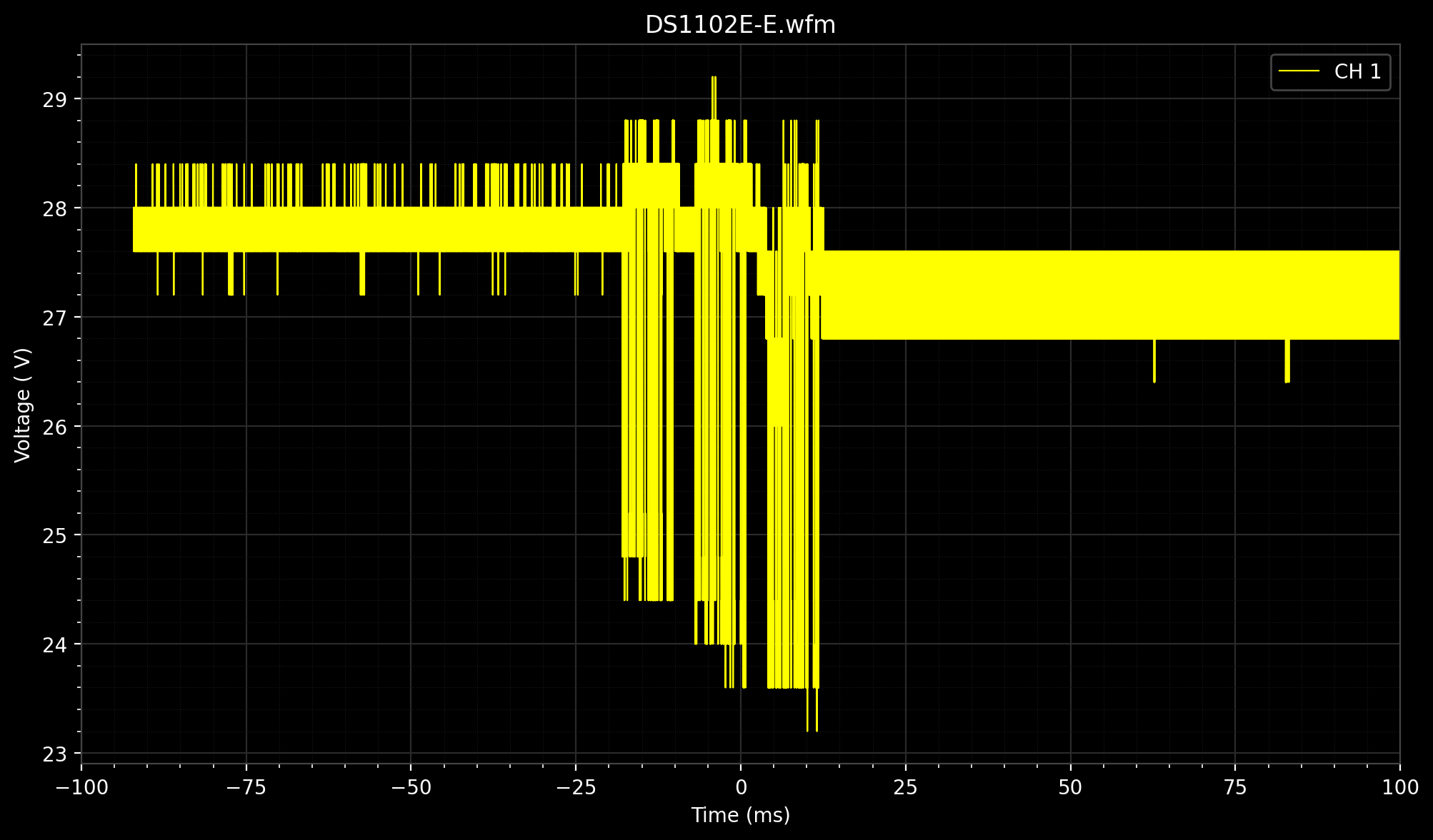
DS1102E-E
[Contributed by @Stapelberg](https://github.com/scottprahl/RigolWFM/issues/11#issue-718562669)
This file uses a 10X probe. First let’s have look at the description of the internal file structure. We see that only channel 1 has been enabled and it has a 10X probe.
[9]:
wfm_url = repo + "wfm/DS1102E-E.wfm?raw=true"
w = Wfm.from_url(wfm_url, "DS1102E")
description = w.describe()
print(description)
downloading 'https://raw.githubusercontent.com/scottprahl/RigolWFM/main/tests/files/wfm/DS1102E-E.wfm?raw=true'
    General:
        File Model   = DS1000E
        User Model   = DS1102E
        Parser Model = wfm1000e
        Firmware     = unknown
        Filename     = DS1102E-E.wfm
        Channels     = [1]

    Trigger:
        Mode     = edge
        Source   = CH1
        Level    = 25.60  V
        Sweep    = SINGLE
        Coupling = DC
        Derived Level     = 24.00  V

     Channel 1:
         Coupling =  unknown
            Scale =    10.00  V/div
           Offset =   -30.80  V
            Probe =      10X
         Inverted =    False

        Time Base =    5.000 ms/div
           Offset =   12.800 ms
            Delta =  200.000 ns/point
           Points =  1048576

         Count    = [        1,        2,        3  ...   1048575,  1048576]
           Raw    = [      132,      132,      132  ...       134,      134]
           Times  = [-92.058 ms,-92.057 ms,-92.057 ms  ... 117.657 ms,117.657 ms]
           Volts  = [ 28.00  V, 28.00  V, 28.00  V  ...  27.20  V, 27.20  V]
[10]:
w.plot()
plt.xlim(-100, 100)
plt.show()
[ ]: