Rigol DS1000Z Waveform Examples
Scott Prahl
Mar 2026
[1]:
%config InlineBackend.figure_format = 'retina'

import numpy as np
import matplotlib.pyplot as plt
import imageio.v3 as iio

from RigolWFM import Wfm, DS1000Z_scopes

repo = "https://raw.githubusercontent.com/scottprahl/RigolWFM/main/tests/files/wfm/"
Honestly, the Rigol firmware for these scopes is a disaster
This should be a trival conversion. The scope stores a series of byte values and there is a scale and offset to convert these to volts. Now for every other Rigol oscilloscope the conversion is
volts = (raw-127)*scale - offset
At least two other people [@michal-szkutnik](https://github.com/michal-szkutnik/pyRigolWfm1000Z) and [@crasu](https://github.com/michal-szkutnik/pyRigolWfm1000Z/issues/3#issue-196373027) have tried to sort this out without apparent success.
So what is the story? Rigol has gone through a series of firmware revisions and things are still not right with the lastest version.
The current status is that the voltage scale seems to be pretty close to correct as long as the scale factor is calculated by
scale = volt_per_division/20
The offset seems to be completely arbitrary. Consequently, if you want to use converted .wfm data, validate it against your own measurement first!
The list of Rigol scopes that probably suffer from the same firmware problems are: DS1074Z-S, DS1104Z, DS1104Z-S, DS1054Z, MSO1054Z, DS1074Z, MSO1074Z, MSO1104Z and the DS1202Z.
[2]:
# Just a couple of handy functions to simplify making comparison graphs.


def plot_compare_one(w, csv_times, csv_data, chno):

    if chno - 1 >= len(w.channels):
        return

    if chno >= len(csv_data):
        return

    ch = w.channels[chno - 1]

    if not ch.enabled:
        return

    plt.figure(num=None, figsize=(12, 6), dpi=80, facecolor="w", edgecolor="k")

    name = w.basename

    plt.title("CH%d: %.3fV/div, %.2fVoff (%s %s) " % (chno, ch.volt_per_division, ch.volt_offset, name, w.firmware))

    plt.plot(csv_times, csv_data[chno], color="green", label="CSV")
    plt.plot(ch.times, ch.volts, color="red", label="WFM")
    plt.xlabel("Time (s)")
    plt.ylabel("Volts")
    plt.grid(True)
    plt.legend(loc="upper right")
    plt.axhline(0, color="black", linestyle=":")

    plt.show()


def plot_compare(w, csv_times, csv_data, toffset=0):
    for i in [1, 2, 3, 4]:
        plot_compare_one(w, csv_times - toffset, csv_data, i)


def scale_plot(w, csv_times, csv_data, chno, scale, v_offset, csv_h_offset, half_ns):

    if chno - 1 >= len(w.channels):
        return

    plt.figure(num=None, figsize=(12, 6), dpi=80, facecolor="w", edgecolor="k")

    ch = w.channels[chno - 1]
    v = ch.volts * scale + v_offset
    vmax = max(v)
    vmin = min(v)
    diff = vmax - vmin
    plt.plot(ch.times * 1e9, v, label=r"$\Delta$V=%.2f (WFM)" % (diff))

    if chno < len(csv_data):
        v = csv_data[chno]
        vmax = max(v)
        vmin = min(v)
        diff = vmax - vmin
        plt.plot(csv_times * 1e9 + csv_h_offset, v, label=r"$\Delta$V=%.2f (CSV)" % (diff))

    name = w.basename
    plt.legend(loc="upper right")
    plt.title("CH%d, %.2fV/div %.2fVoff (%s %s)" % (chno, ch.volt_per_division, ch.volt_offset, name, w.firmware))
    plt.xlim(-half_ns, half_ns)
    plt.axhline(0, color="black", linestyle=":")
    plt.show()


#    print("       volt/division = %.4f" % (ch.volt_per_division))
#    print("  (volt/division)/20 = %.4f" % (ch.volt_per_division/20.0))
#    print("             y_scale = %.4f" % (ch.y_scale))
#    print("     %.3f * y_scale = %.4f (actual value)" % (scale, ch.y_scale*scale))
#    print("(volt/division)/21.0 = %.4f" % (-ch.volt_per_division/21))
A list of Rigol scopes in the DS1000Z family is:
[3]:
print(DS1000Z_scopes)
['Z', '1000Z', 'DS1000Z', 'DS1202Z', 'DS1054Z', 'MSO1054Z', 'DS1074Z', 'MSO1074Z', 'DS1074Z-S', 'DS1104Z', 'MSO1104Z', 'DS1104Z-S']
Background on the voltage and time conversions.
It is bit confusing because the .wfm files and the .csv files can differ. I think that the .wfm files always correspond to the scope’s RAW mode and the .csv files can be limited to just the display or NORMAL mode.
Voltage conversion
From the Rigol Programming Guide
page 2-221
volts = (raw_byte - YORigin - YREFerence) * YINCrement
page 2-223, assuming RAW mode
YINCrement = VerticalScale/25 YORigin = VerticalOffset/YINCrement YREFerence is always 127
So this becomes
volts = (raw_byte - VerticalOffset/YINCrement - 127) * YINCrement volts = (raw_byte - 127) * YINCrement - VerticalOffset
volts = (raw_byte - 127) * VerticalScale/25 - VerticalOffset
and this can be interpreted as
volts = (raw_byte - 127.0) * VoltsPerDivision/25.0 - VerticalOffset
Where the decimal points are needed to force python avoid integer math.
Now based on actually comparing DS1054Z .wfm data with .csv data, the above equation fails. This is unfortunate because this is the equation used all other Rigol scopes. Instead the equation is something like
volts = (raw_byte - 127) * (-VerticalScale/20) - VerticalOffset + VerticalScale
Gaak.
Time Conversions
On page 2-222 we find that
XINCrement the time difference between two neighboring points of the specified channel source in the X direction and
XINCrement = 1/SampleRate
on the other hand, when the scope is in NORMAL mode or display mode, then
XINCrement = TimeScale/100
XORigin is the start time of the waveform data of the channel source currently selected in the X direction.
Both should be in seconds.
CSV Files
Display saving
It seems that the time parameters provided in the .csv file (when saving the display points) is set so the center point is at time zero. There are twelve divisions that are saved and each division has 100 points. Therefore the time increment is given by
time_increment = time_per_division/100
and the start time is
-600 * time_increment
(There is probably an time offset also …)
Start with waveform with a single trace
[Contributed by @JBR48](https://github.com/michal-szkutnik/pyRigolWfm1000Z/issues/1#issuecomment-212646090)
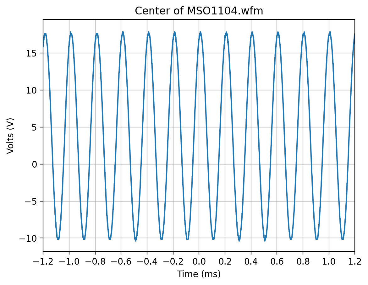
First let’s look at the description of the internal file structure. We see that only channel 1 has been enabled. Unfortunately, there is not an accompanying .csv file so we cannot do much more than verify that the file is parsed and displays a plausible 5kHz sine wave.
[4]:
# raw=true is needed because this is a binary file
wfm_url = repo + "MSO1104.wfm" + "?raw=true"

w = Wfm.from_url(wfm_url, "1000Z")

description = w.describe()
print(description)
    General:
        File Model   = MSO1104Z
        User Model   = 1000Z
        Parser Model = wfm1000z
        Firmware     = 00.04.03.SP2
        Filename     = MSO1104.wfm
        Channels     = [1]

    Trigger:
        Derived Level (CH1) = 3.35  V

     Channel 1:
         Coupling =       AC
            Scale =     5.00  V/div
           Offset =   400.00 mV
            Probe =      10X
         Inverted =    False

        Time Base =    1.000 ms/div
           Offset = -200.000 ps
            Delta = 1000.000 ns/point
           Points =  1200512

         Count    = [        1,        2,        3  ...   1200511,  1200512]
           Raw    = [      174,      175,      176  ...        70,       70]
           Times  = [-600.256 ms,-600.255 ms,-600.254 ms  ... 600.254 ms,600.255 ms]
           Volts  = [ 16.35  V, 16.60  V, 16.85  V  ...  -9.65  V, -9.65  V]
downloading 'https://raw.githubusercontent.com/scottprahl/RigolWFM/main/tests/files/wfm/MSO1104.wfm?raw=true'
[5]:
ch = w.channels[0]
plt.plot(ch.times * 1e3 - 0.04, ch.volts)
plt.xlabel("Time (ms)")
plt.ylabel("Volts (V)")
plt.xlim(-1.2, 1.2)
plt.title("Center of MSO1104.wfm")
plt.xticks(np.linspace(-1.2, 1.2, 13))
plt.grid(True)
plt.show()
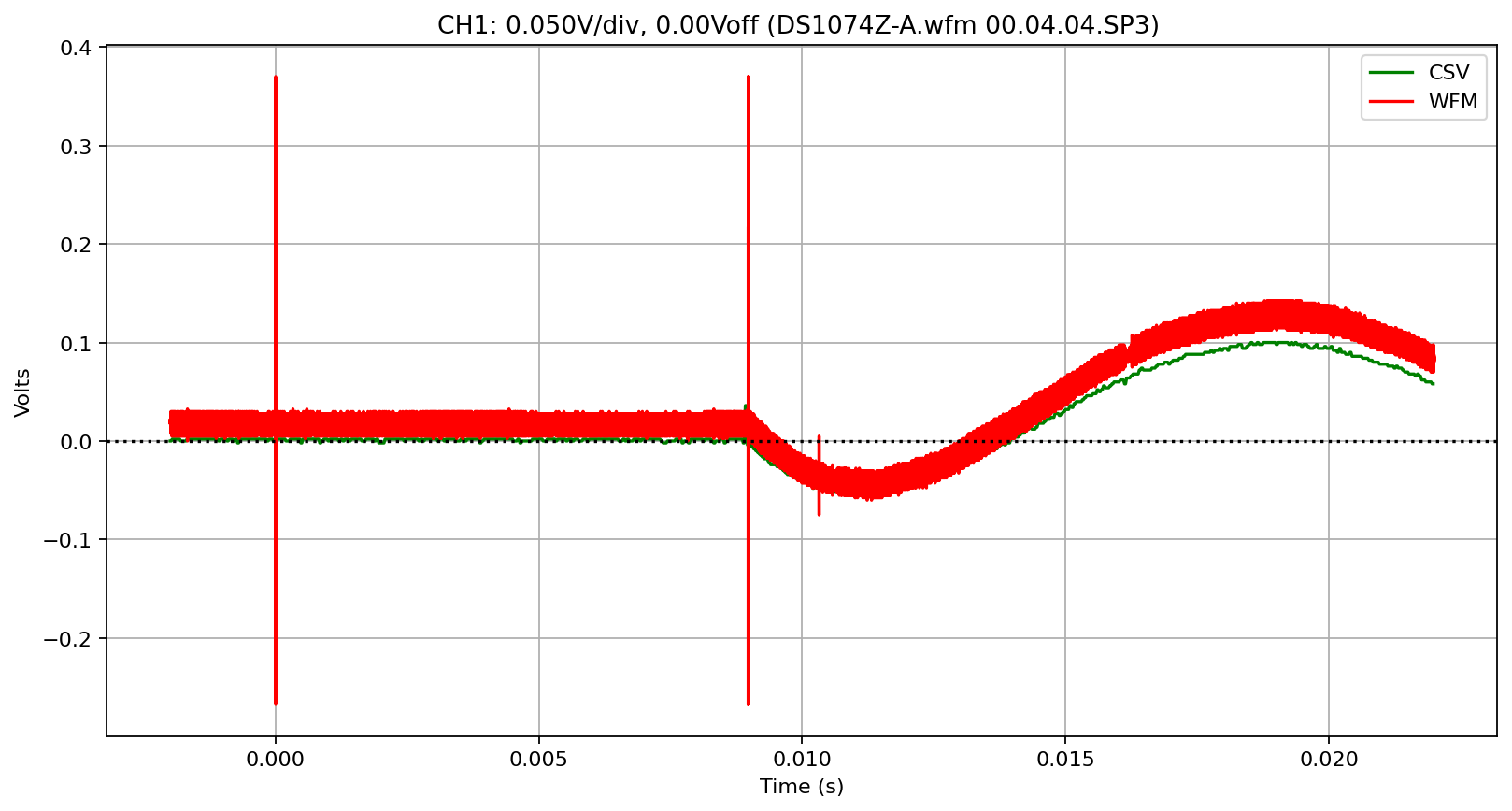
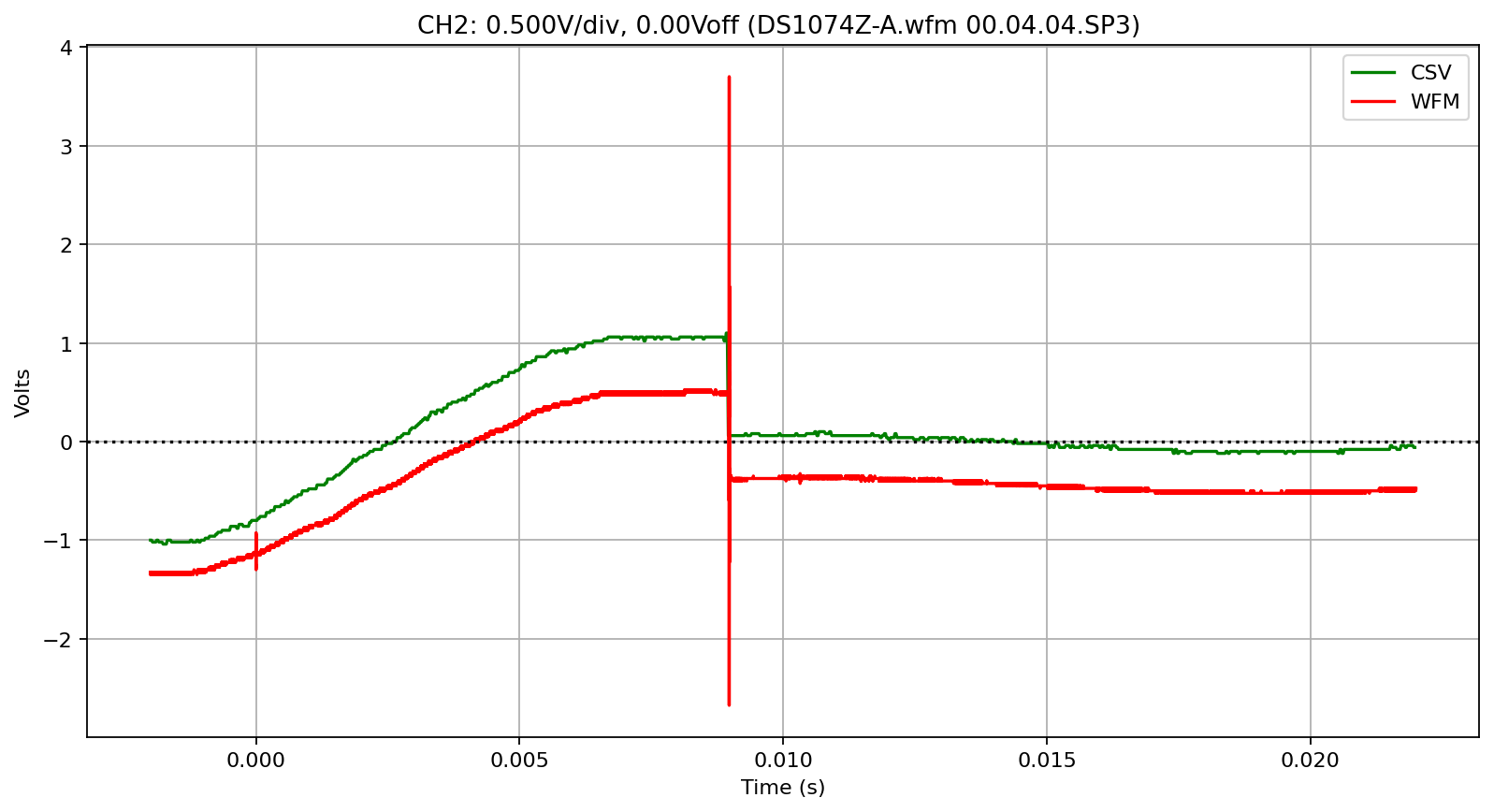
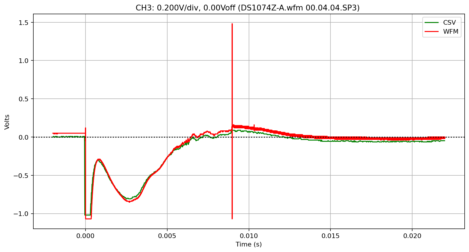
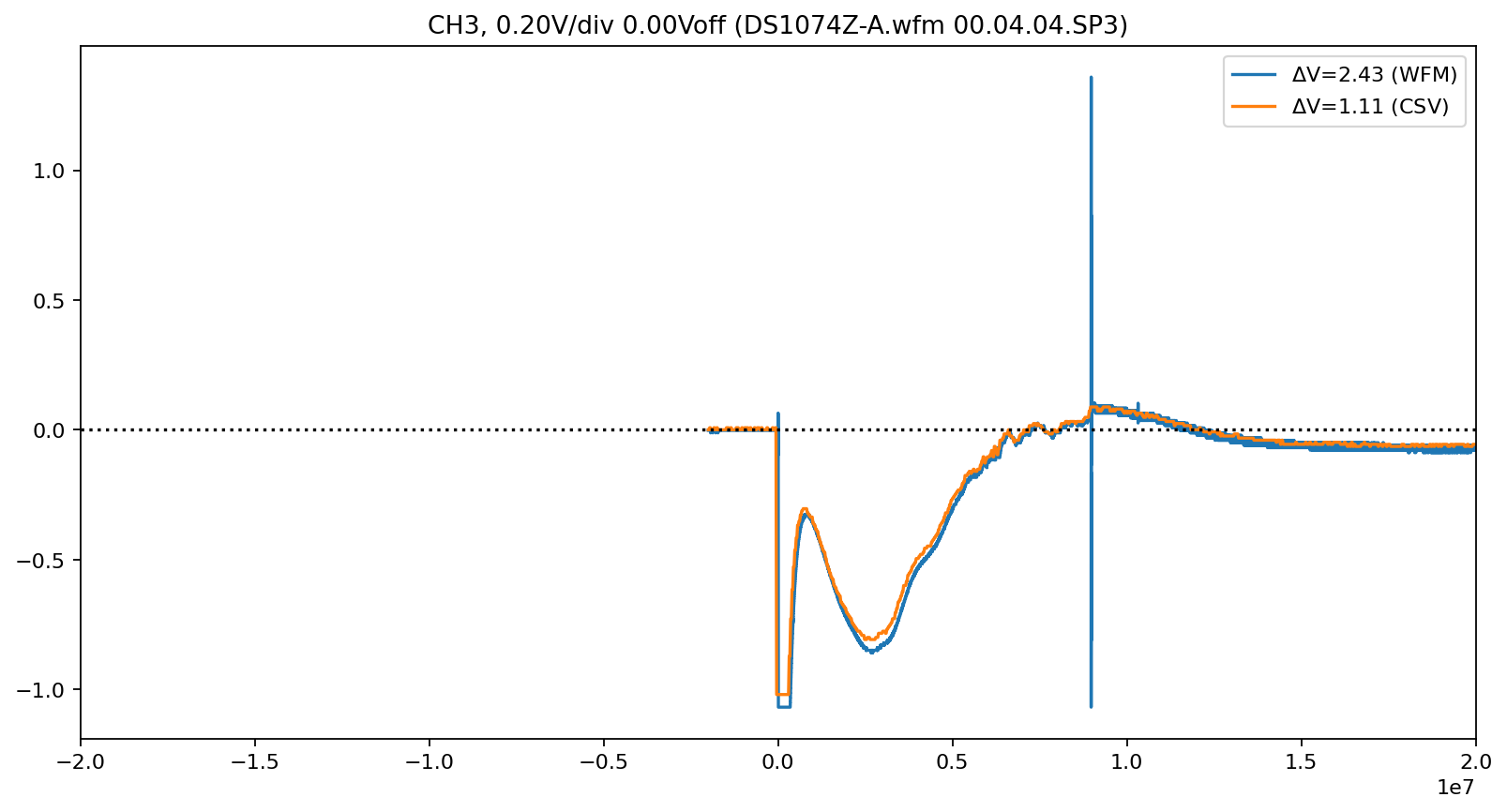
DS1074Z-A Scope file
[Contributed by @ro-bercik](https://github.com/michal-szkutnik/pyRigolWfm1000Z/issues/4#issue-361649641)
Note that this file uses old 04.04.SP3 firmware and both the offset and scaling is a bit off. Specifically, it looks like the scaling factor (usually, volts_per_division/20) is (usually, volts_per_division/21).
[6]:
name = "DS1074Z-A"
wfm_url = repo + name + ".wfm" + "?raw=true"
w = Wfm.from_url(wfm_url, "1000Z")
downloading 'https://raw.githubusercontent.com/scottprahl/RigolWFM/main/tests/files/wfm/DS1074Z-A.wfm?raw=true'
[7]:
csv_filename = repo + name + ".csv"
csv_data = np.genfromtxt(csv_filename, delimiter=",", skip_header=2)
csv_data = csv_data[:, :-1].T

t_incr = 2.000000e-05  # seconds/point
t_start = -len(csv_data[0]) / 2.0 * t_incr  # seconds so that t=0 is in the center
csv_times = csv_data[0] * t_incr + t_start  # seconds

print(w.describe())
    General:
        File Model   = DS1074Z
        User Model   = 1000Z
        Parser Model = wfm1000z
        Firmware     = 00.04.04.SP3
        Filename     = DS1074Z-A.wfm
        Channels     = [1, 2, 3]

    Trigger:
        Derived Level (CH1) = 15.00 mV
        Derived Level (CH2) = -1.12  V
        Derived Level (CH3) = 50.00 mV

     Channel 1:
         Coupling =       AC
            Scale =    50.00 mV/div
           Offset =     0.00  V
            Probe =       1X
         Inverted =    False

        Time Base =    2.000 ms/div
           Offset =   10.000 ms
            Delta =    8.000 ns/point
           Points =  3000128

         Count    = [        1,        2,        3  ...   3000127,  3000128]
           Raw    = [      115,      115,      115  ...       140,      140]
           Times  = [-2.001 ms,-2.001 ms,-2.000 ms  ... 22.000 ms,22.001 ms]
           Volts  = [ 20.00 mV, 20.00 mV, 20.00 mV  ...  82.50 mV, 82.50 mV]

     Channel 2:
         Coupling =       AC
            Scale =   500.00 mV/div
           Offset =     0.00  V
            Probe =       1X
         Inverted =    False

        Time Base =    2.000 ms/div
           Offset =   10.000 ms
            Delta =    8.000 ns/point
           Points =  3000128

         Count    = [        1,        2,        3  ...   3000127,  3000128]
           Raw    = [       54,       53,       54  ...        88,       88]
           Times  = [-2.001 ms,-2.001 ms,-2.000 ms  ... 22.000 ms,22.001 ms]
           Volts  = [ -1.33  V, -1.35  V, -1.33  V  ... -475.00 mV,-475.00 mV]

     Channel 3:
         Coupling =       AC
            Scale =   200.00 mV/div
           Offset =     0.00  V
            Probe =       1X
         Inverted =    False

        Time Base =    2.000 ms/div
           Offset =   10.000 ms
            Delta =    8.000 ns/point
           Points =  3000128

         Count    = [        1,        2,        3  ...   3000127,  3000128]
           Raw    = [      112,      112,      112  ...       106,      106]
           Times  = [-2.001 ms,-2.001 ms,-2.000 ms  ... 22.000 ms,22.001 ms]
           Volts  = [ 50.00 mV, 50.00 mV, 50.00 mV  ... -10.00 mV,-10.00 mV]
[8]:
plot_compare(w, csv_times, csv_data, -0.01)
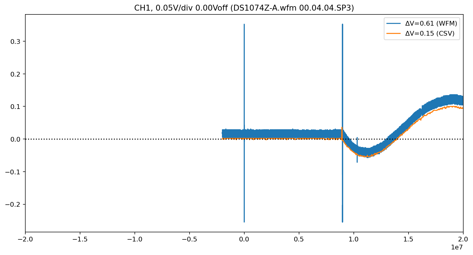
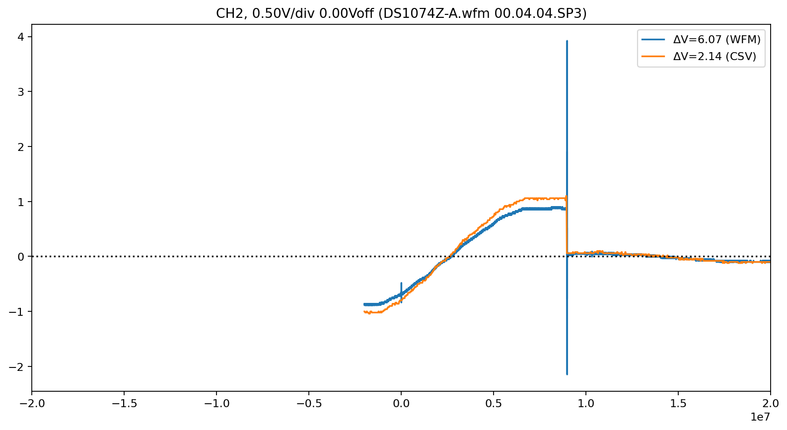
[9]:
scale = 0.952
end_ns = 20000000
scale_plot(w, csv_times, csv_data, 1, scale, 0.0, end_ns / 2, end_ns)
scale_plot(w, csv_times, csv_data, 2, scale, 0.4, end_ns / 2, end_ns)
scale_plot(w, csv_times, csv_data, 3, scale, -0.05, end_ns / 2, end_ns)
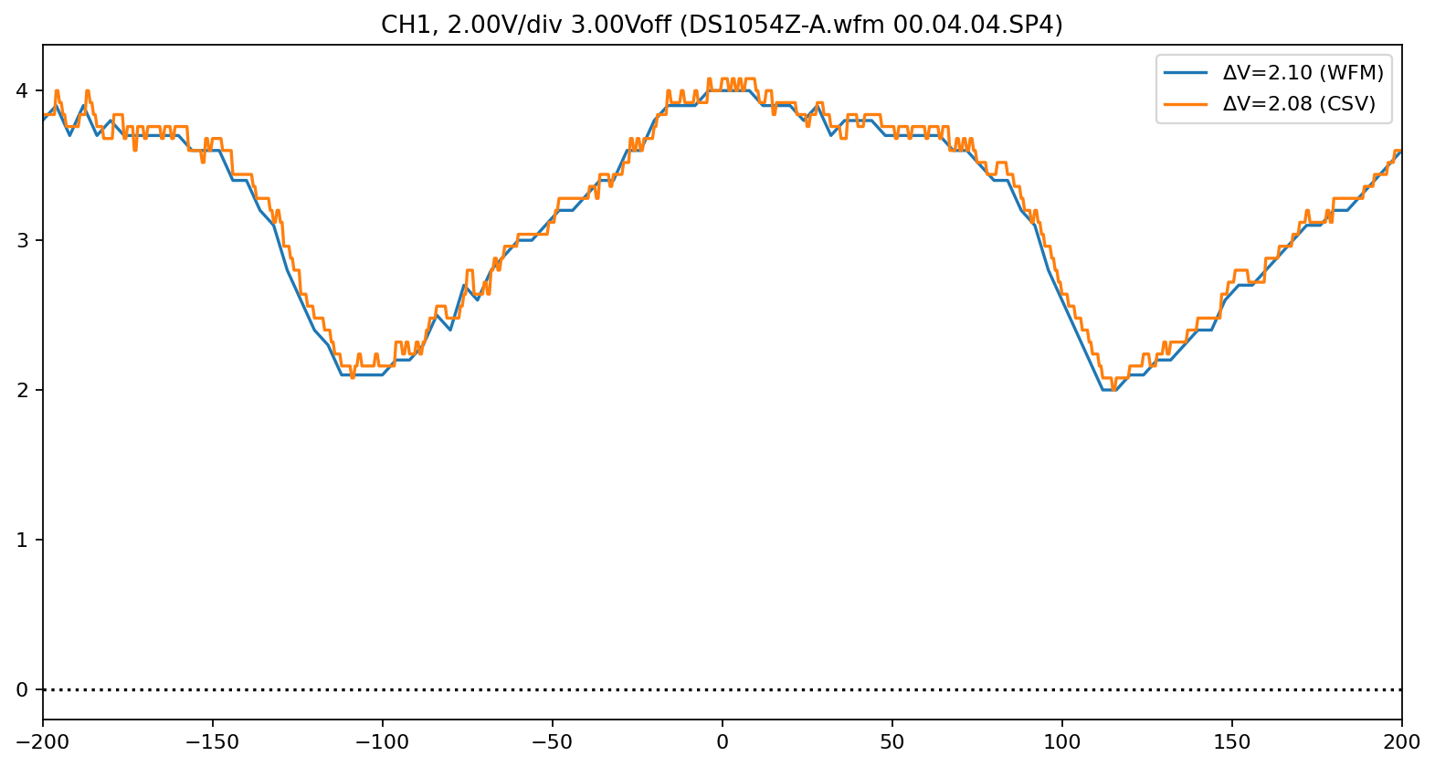
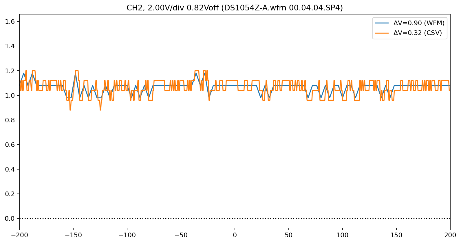
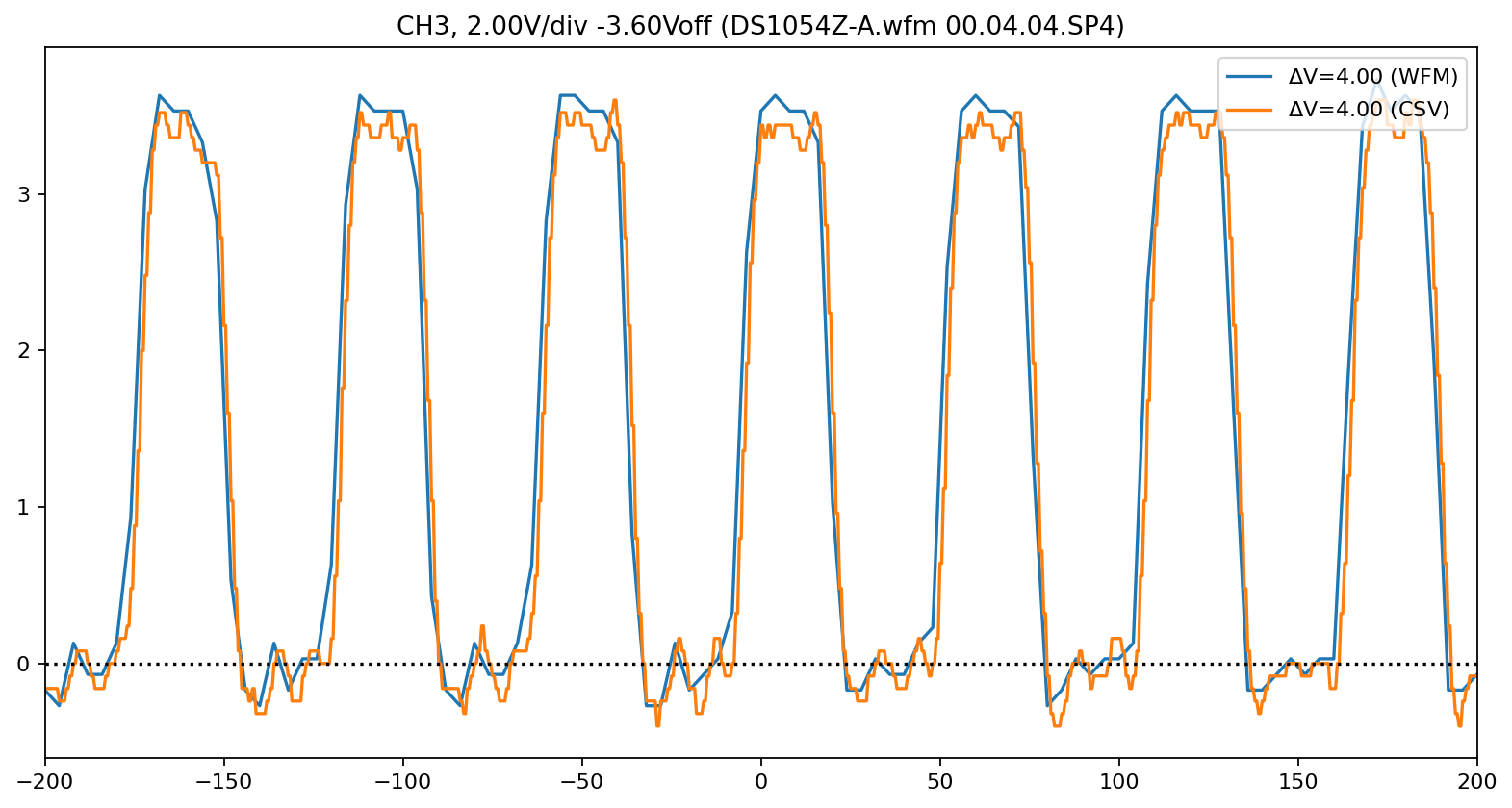
DS1054Z-A Scope file
[Contributed by @JensRestemeier](https://github.com/scottprahl/RigolWFM/issues/5#issuecomment-599158528)
[10]:
name = "DS1054Z-A"
wfm_url = repo + name + ".wfm" + "?raw=true"
w = Wfm.from_url(wfm_url, "1000Z")

csv_filename = repo + name + ".csv"
csv_data = np.genfromtxt(csv_filename, delimiter=",", skip_header=2)
csv_data = csv_data[:, :-1].T


t_incr = 5.000000e-10  # seconds/point
t_start = -len(csv_data[0]) / 2.0 * t_incr  # seconds so that t=0 is in the center
csv_times = csv_data[0] * t_incr + t_start  # seconds
print(w.describe())
General:
File Model = DS1054Z
User Model = 1000Z
Parser Model = wfm1000z
Firmware = 00.04.04.SP4
Filename = DS1054Z-A.wfm
Channels = [1, 2, 3, 4]
Trigger:
Derived Level (CH1) = 4.00 V
Derived Level (CH2) = 880.00 mV
Derived Level (CH3) = 3.20 V
Derived Level (CH4) = -2.89 V
Channel 1:
Coupling = DC
Scale = 2.00 V/div
Offset = 3.00 V
Probe = 10X
Inverted = False
Time Base = 50.000 ns/div
Offset = 0.000 s
Delta = 4.000 ns/point
Points = 278
Count = [ 1, 2, 3 ... 277, 278]
Raw = [ 158, 157, 159 ... 176, 176]
Times = [-556.000 ns,-552.000 ns,-548.000 ns ... 548.000 ns,552.000 ns]
Volts = [ 2.10 V, 2.00 V, 2.20 V ... 3.90 V, 3.90 V]
Channel 2:
Coupling = DC
Scale = 2.00 V/div
Offset = 820.00 mV
Probe = 10X
Inverted = False
Time Base = 50.000 ns/div
Offset = 0.000 s
Delta = 4.000 ns/point
Points = 278
Count = [ 1, 2, 3 ... 277, 278]
Raw = [ 124, 123, 124 ... 128, 129]
Times = [-556.000 ns,-552.000 ns,-548.000 ns ... 548.000 ns,552.000 ns]
Volts = [880.00 mV,780.00 mV,880.00 mV ... 1.28 V, 1.38 V]
Channel 3:
Coupling = DC
Scale = 2.00 V/div
Offset = -3.60 V
Probe = 10X
Inverted = False
Time Base = 50.000 ns/div
Offset = 0.000 s
Delta = 4.000 ns/point
Points = 278
Count = [ 1, 2, 3 ... 277, 278]
Raw = [ 103, 103, 102 ... 102, 104]
Times = [-556.000 ns,-552.000 ns,-548.000 ns ... 548.000 ns,552.000 ns]
Volts = [ 3.20 V, 3.20 V, 3.10 V ... 3.10 V, 3.30 V]
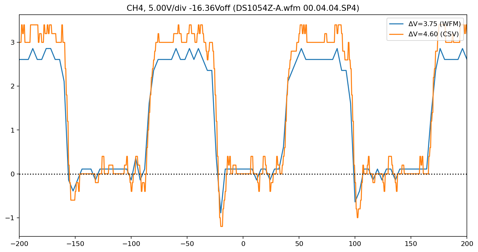
Channel 4:
Coupling = DC
Scale = 5.00 V/div
Offset = -16.36 V
Probe = 10X
Inverted = False
Time Base = 50.000 ns/div
Offset = 0.000 s
Delta = 4.000 ns/point
Points = 278
Count = [ 1, 2, 3 ... 277, 278]
Raw = [ 41, 40, 40 ... 28, 28]
Times = [-556.000 ns,-552.000 ns,-548.000 ns ... 548.000 ns,552.000 ns]
Volts = [-140.00 mV,-390.00 mV,-390.00 mV ... -3.39 V, -3.39 V]
downloading 'https://raw.githubusercontent.com/scottprahl/RigolWFM/main/tests/files/wfm/DS1054Z-A.wfm?raw=true'
[11]:
scale = 1
end_ns = 200
offset_ns = -62
scale_plot(w, csv_times, csv_data, 1, scale, 0.0, offset_ns, end_ns)
scale_plot(w, csv_times, csv_data, 2, scale, 0.2, offset_ns, end_ns)
scale_plot(w, csv_times, csv_data, 3, scale, 0.33, offset_ns, end_ns)
scale_plot(w, csv_times, csv_data, 4, scale, 3, offset_ns, end_ns)
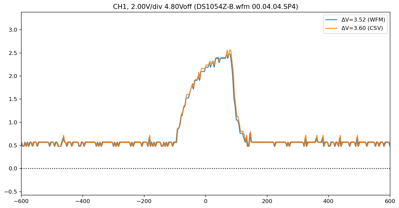
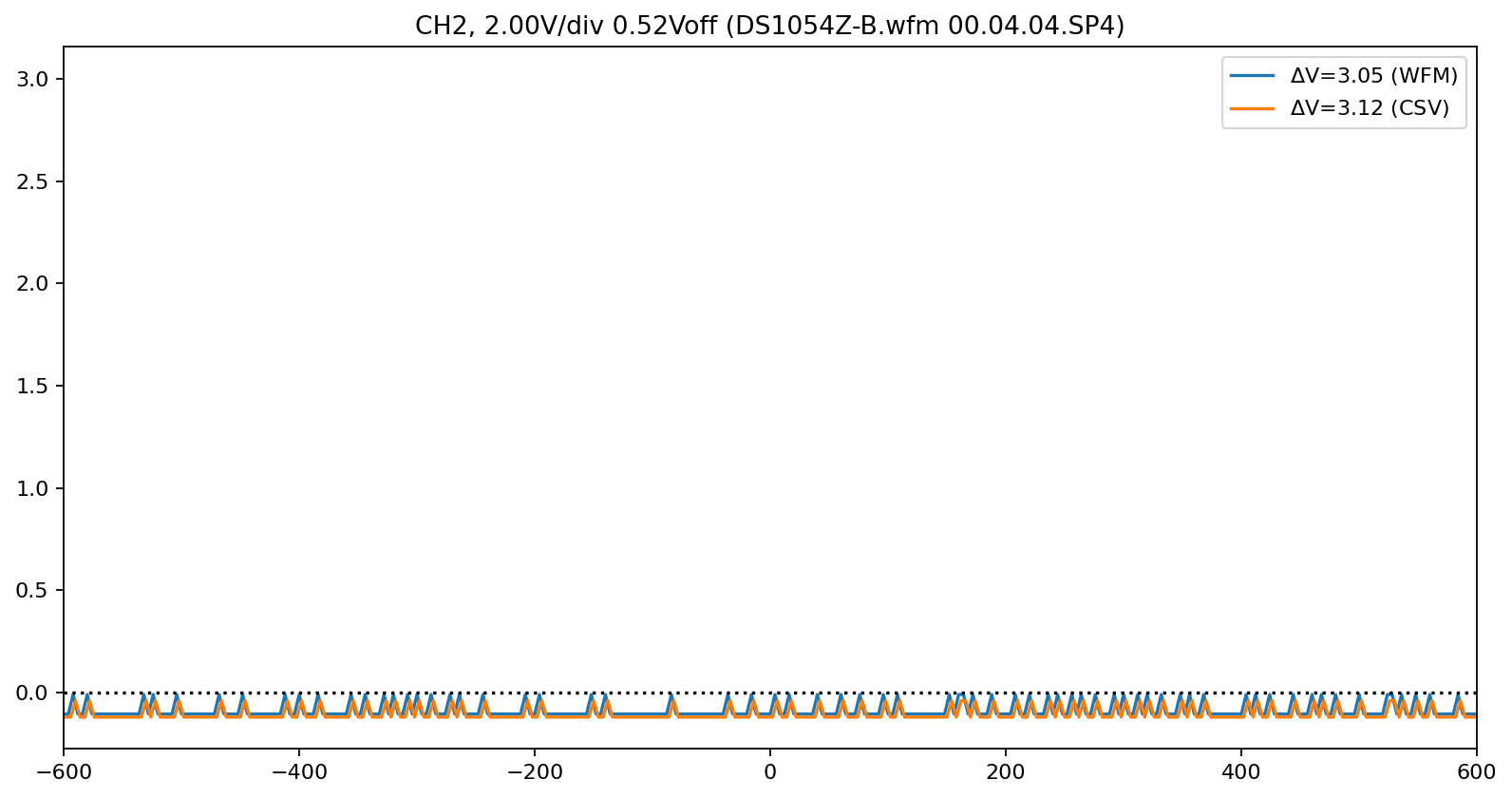
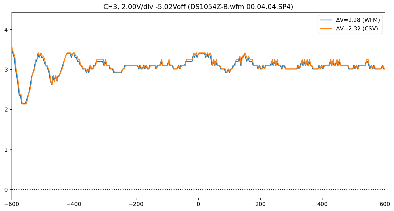
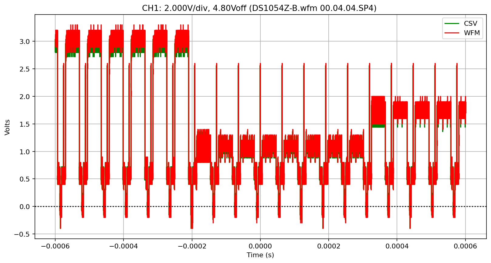
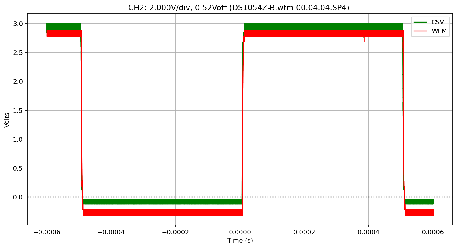
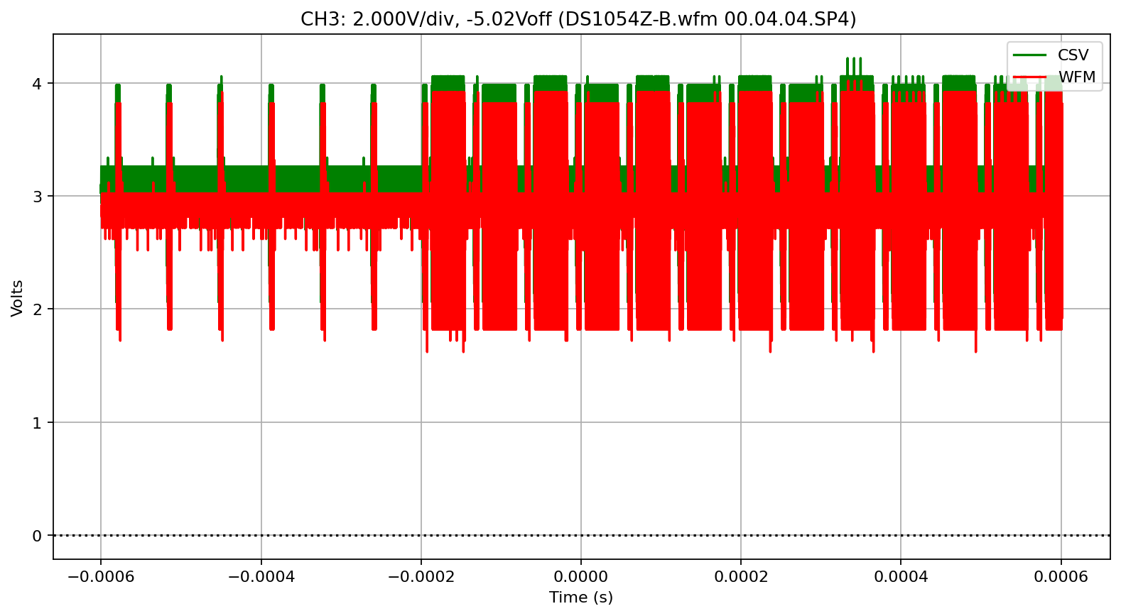
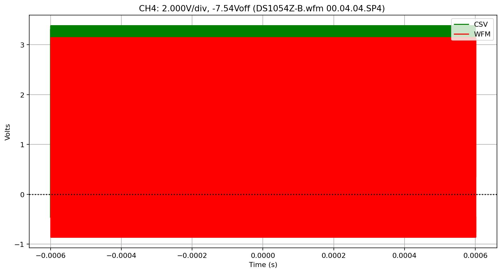
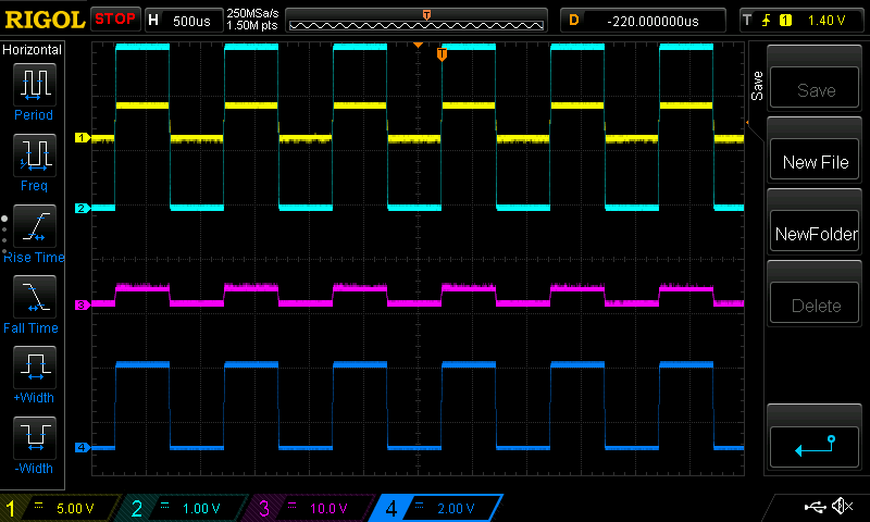
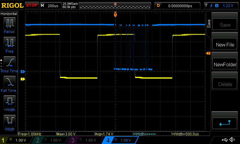
DS1054Z-B Scope file
[Contributed by @JensRestemeier](https://github.com/scottprahl/RigolWFM/issues/5#issuecomment-599210113)
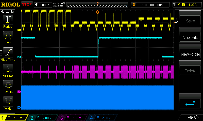
https://raw.githubusercontent.com/scottprahl/RigolWFM/main/tests/files/wfm/DS1054Z-B.png
[12]:
name = "DS1054Z-B"
wfm_url = repo + name + ".wfm" + "?raw=true"
w = Wfm.from_url(wfm_url, "1000Z")

csv_filename = repo + name + ".csv"
csv_data = np.genfromtxt(csv_filename, delimiter=",", skip_header=2)
csv_data = csv_data[:, :-1].T

t_incr = 4.000000e-9  # seconds/point
t_start = -len(csv_data[0]) / 2.0 * t_incr  # seconds so that t=0 is in the center
csv_times = csv_data[0] * t_incr + t_start  # seconds
downloading 'https://raw.githubusercontent.com/scottprahl/RigolWFM/main/tests/files/wfm/DS1054Z-B.wfm?raw=true'
[13]:
scale = 0.952
end_ns = 600
offset_ns = 918
scale_plot(w, csv_times, csv_data, 1, scale, 0.0, offset_ns, end_ns)
scale_plot(w, csv_times, csv_data, 2, scale, 0.2, offset_ns, end_ns)
scale_plot(w, csv_times, csv_data, 3, scale, 0.33, offset_ns, end_ns)
scale_plot(w, csv_times, csv_data, 4, scale, 0.38, offset_ns, end_ns)

[14]:
plot_compare(w, csv_times, csv_data, 0)
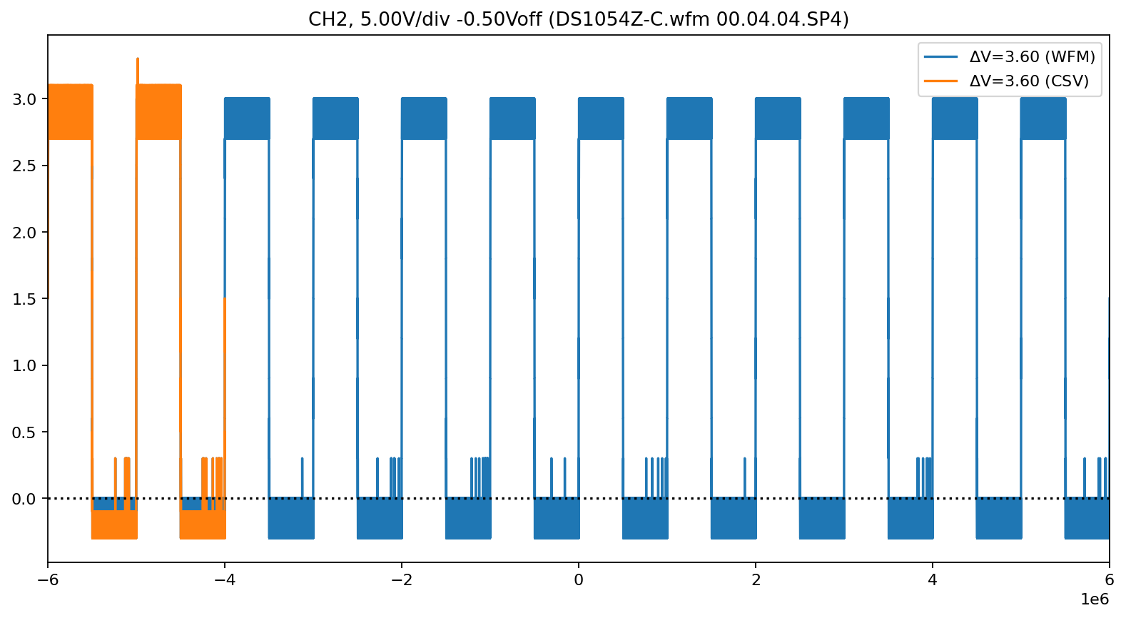
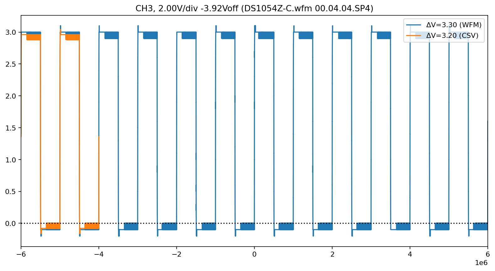
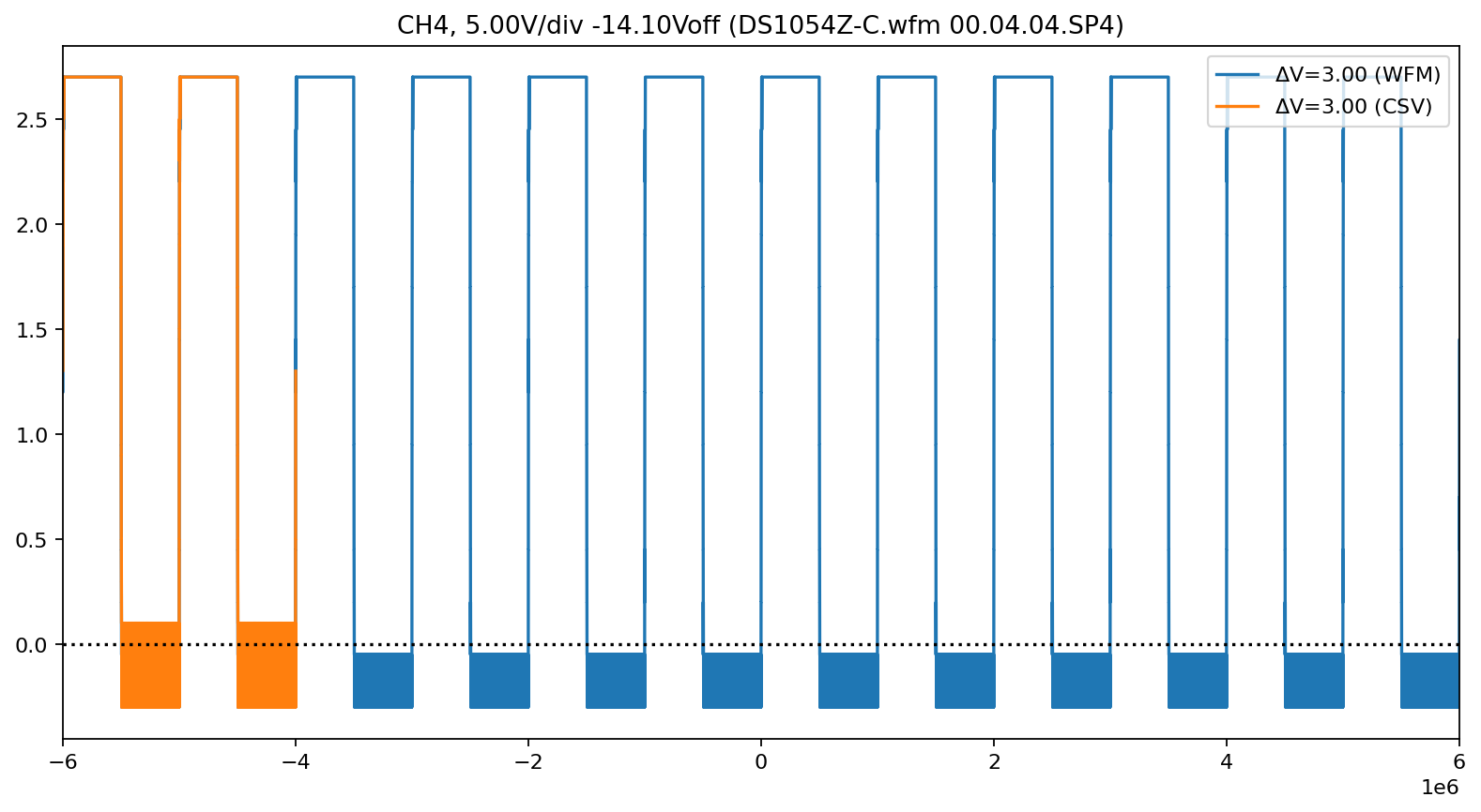
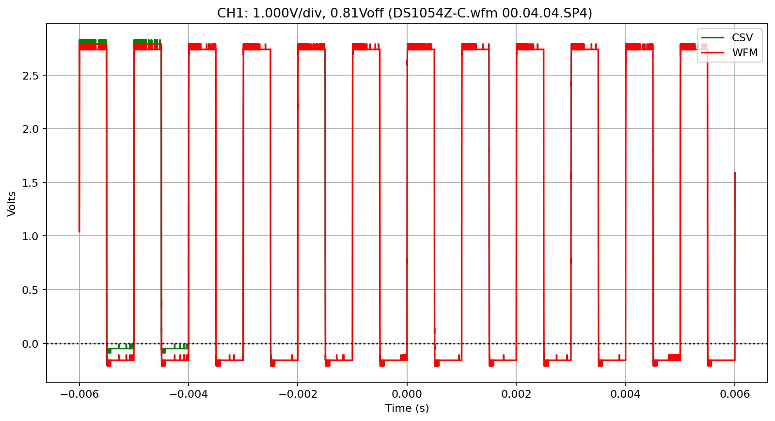
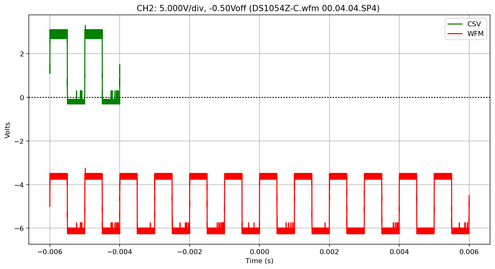
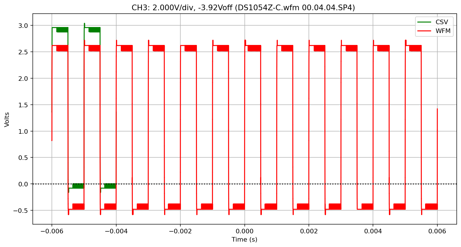
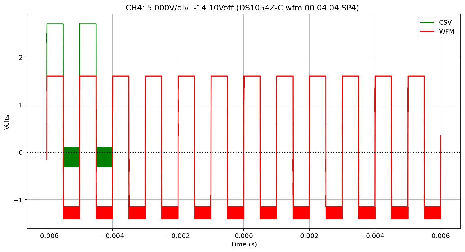
DS1054Z-C Scope file
[Contributed by @electronoob.](https://github.com/scottprahl/RigolWFM/issues/5#issuecomment-600314960)
[15]:
name = "DS1054Z-C"
wfm_url = repo + name + ".wfm" + "?raw=true"
w = Wfm.from_url(wfm_url, "1000Z")

csv_filename = repo + name + ".csv"
csv_data = np.genfromtxt(csv_filename, delimiter=",", skip_header=2)
csv_data = csv_data[:, :-1].T

# this .csv file has the last 250000 points removed
t_incr = 4.000000e-9  # seconds/point
t_start = -len(csv_data[0]) / 2.0 * t_incr  # seconds so that t=0 is in the center
csv_times = csv_data[0] * t_incr + t_start  # seconds
downloading 'https://raw.githubusercontent.com/scottprahl/RigolWFM/main/tests/files/wfm/DS1054Z-C.wfm?raw=true'
[16]:
scale = 1
end_ns = 6000000
offset_ns = -77 - 5000000
scale_plot(w, csv_times, csv_data, 1, scale, 0.1, offset_ns, end_ns)
scale_plot(w, csv_times, csv_data, 2, scale * 1.2, 7.2, offset_ns, end_ns)
scale_plot(w, csv_times, csv_data, 3, scale, 0.38, offset_ns, end_ns)
scale_plot(w, csv_times, csv_data, 4, scale, 1.1, offset_ns, end_ns)
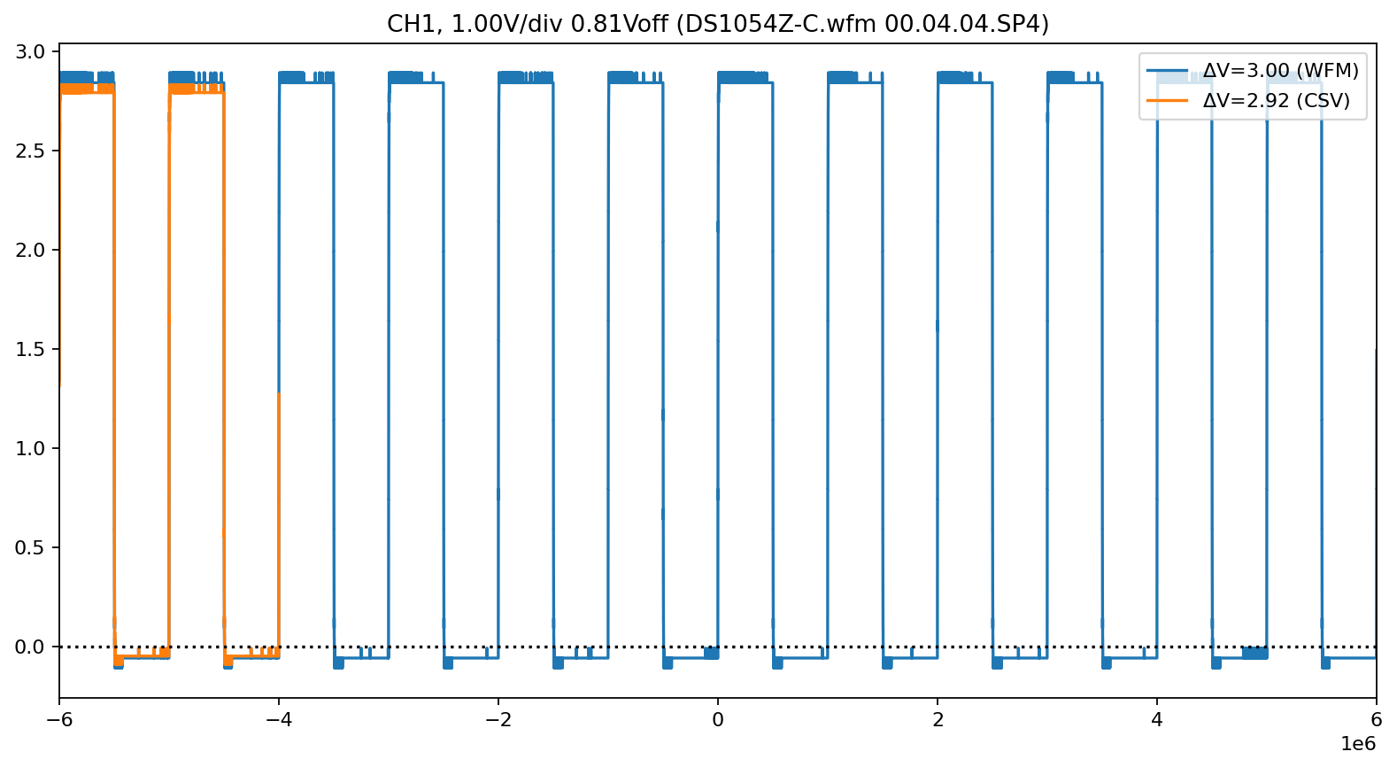
[17]:
plot_compare(w, csv_times, csv_data, 0.005)
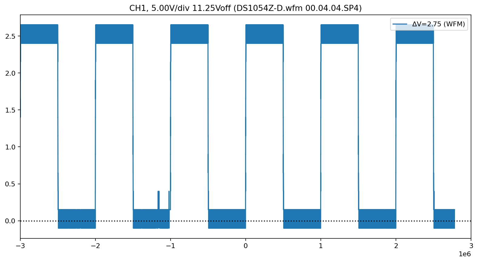
DS1054Z-D Scope file
[Contributed by @JensRestemeier](https://github.com/scottprahl/RigolWFM/issues/5#issuecomment-602181223)
[18]:
name = "DS1054Z-D"
wfm_url = repo + name + ".wfm" + "?raw=true"
w = Wfm.from_url(wfm_url, "1000Z")

csv_filename = repo + name + ".csv"
csv_data = np.genfromtxt(csv_filename, delimiter=",", skip_header=2)
csv_data = csv_data[:, :-1].T

t_incr = 4.000000e-9  # seconds/point
t_start = -len(csv_data[0]) / 2.0 * t_incr  # seconds so that t=0 is in the center
csv_times = csv_data[0] * t_incr + t_start  # seconds
downloading 'https://raw.githubusercontent.com/scottprahl/RigolWFM/main/tests/files/wfm/DS1054Z-D.wfm?raw=true'
[19]:
print(w.describe())
    General:
        File Model   = DS1054Z
        User Model   = 1000Z
        Parser Model = wfm1000z
        Firmware     = 00.04.04.SP4
        Filename     = DS1054Z-D.wfm
        Channels     = [1, 2, 3, 4]

    Trigger:
        Derived Level (CH1) = -6.50  V
        Derived Level (CH2) = 1.66  V
        Derived Level (CH3) = -8.50  V
        Derived Level (CH4) = 1.34  V

     Channel 1:
         Coupling =       DC
            Scale =     5.00  V/div
           Offset =    11.25  V
            Probe =      10X
         Inverted =    False

        Time Base =  500.000 µs/div
           Offset = -220.000 µs
            Delta =    4.000 ns/point
           Points =  1500128

         Count    = [        1,        2,        3  ...   1500127,  1500128]
           Raw    = [      121,      120,      121  ...       121,      121]
           Times  = [-3.220 ms,-3.220 ms,-3.220 ms  ...  2.780 ms, 2.780 ms]
           Volts  = [ -7.75  V, -8.00  V, -7.75  V  ...  -7.75  V, -7.75  V]

     Channel 2:
         Coupling =       DC
            Scale =     1.00  V/div
           Offset =   940.00 mV
            Probe =      10X
         Inverted =    False

        Time Base =  500.000 µs/div
           Offset = -220.000 µs
            Delta =    4.000 ns/point
           Points =  1500128

         Count    = [        1,        2,        3  ...   1500127,  1500128]
           Raw    = [      123,      124,      124  ...       124,      124]
           Times  = [-3.220 ms,-3.220 ms,-3.220 ms  ...  2.780 ms, 2.780 ms]
           Volts  = [-140.00 mV,-90.00 mV,-90.00 mV  ... -90.00 mV,-90.00 mV]

     Channel 3:
         Coupling =       DC
            Scale =    10.00  V/div
           Offset =    -8.50  V
            Probe =      10X
         Inverted =    False

        Time Base =  500.000 µs/div
           Offset = -220.000 µs
            Delta =    4.000 ns/point
           Points =  1500128

         Count    = [        1,        2,        3  ...   1500127,  1500128]
           Raw    = [       70,       70,       70  ...        70,       70]
           Times  = [-3.220 ms,-3.220 ms,-3.220 ms  ...  2.780 ms, 2.780 ms]
           Volts  = [-10.00  V,-10.00  V,-10.00  V  ... -10.00  V,-10.00  V]

     Channel 4:
         Coupling =       DC
            Scale =     2.00  V/div
           Offset =    -6.94  V
            Probe =      10X
         Inverted =    False

        Time Base =  500.000 µs/div
           Offset = -220.000 µs
            Delta =    4.000 ns/point
           Points =  1500128

         Count    = [        1,        2,        3  ...   1500127,  1500128]
           Raw    = [       33,       33,       33  ...        33,       33]
           Times  = [-3.220 ms,-3.220 ms,-3.220 ms  ...  2.780 ms, 2.780 ms]
           Volts  = [-460.00 mV,-460.00 mV,-460.00 mV  ... -460.00 mV,-460.00 mV]
[20]:
plot_compare(w, csv_times, csv_data, toffset=0)
[21]:
scale = 1.0
end_ns = 3000000
offset_ns = -220100

scale_plot(w, csv_times, csv_data, 1, scale, 7.9, offset_ns, end_ns)
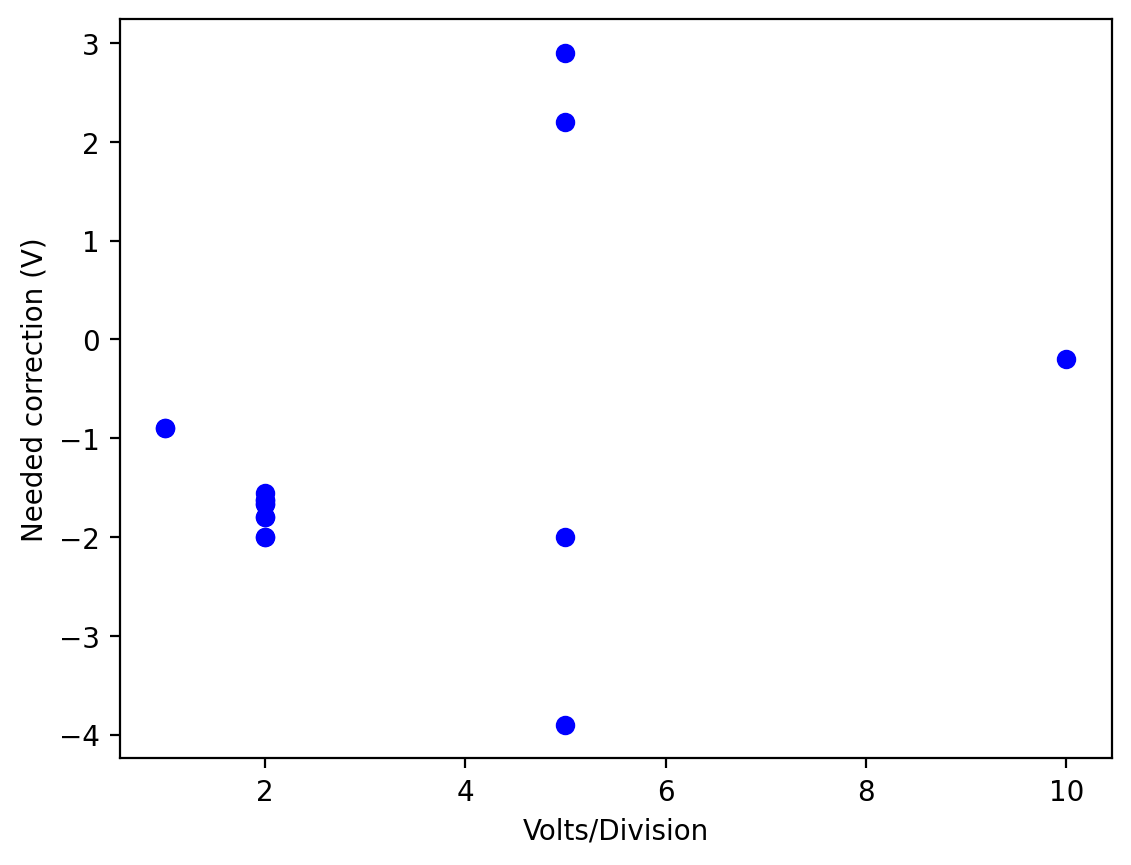
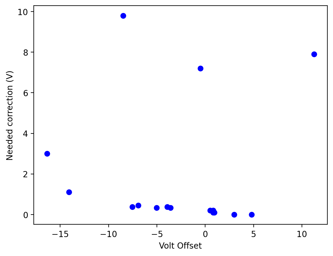
Summarizing all the results
It is not pretty. If there was anything consistent, then it is not apparent to me!
[22]:
vd = np.array([2, 2, 2, 5, 2, 2, 2, 2, 1, 5, 2, 5, 5, 1, 10, 2])
voff = np.array([3, 0.82, -3.6, -16.36, 4.8, 0.52, -5.02, -7.54, 0.81, -0.5, -3.92, -14.1, 11.25, 0.94, -8.5, -6.94])
yoff = voff - vd
vcorrect = np.array([0, 0.2, 0.33, 3, 0, 0.2, 0.33, 0.38, 0.1, 7.2, 0.38, 1.1, 7.9, 0.1, 9.8, 0.45])
plt.plot(vd, vcorrect - vd, "ob")
plt.xlabel("Volts/Division")
plt.ylabel("Needed correction (V)")
plt.show()

plt.plot(voff, vcorrect, "ob")
plt.xlabel("Volt Offset")
plt.ylabel("Needed correction (V)")
plt.show()
Testing channel selection
[23]:
name = "DS1054Z-A"
wfm_url = repo + name + ".wfm" + "?raw=true"
w = Wfm.from_url(wfm_url, "1000Z", selected="24")

csv_filename = repo + name + ".csv"
csv_data = np.genfromtxt(csv_filename, delimiter=",", skip_header=2)
csv_data = csv_data[:, :-1].T


t_incr = 5.000000e-10  # seconds/point
t_start = -len(csv_data[0]) / 2.0 * t_incr  # seconds so that t=0 is in the center
csv_times = csv_data[0] * t_incr + t_start  # seconds
print(w.describe())
    General:
        File Model   = DS1054Z
        User Model   = 1000Z
        Parser Model = wfm1000z
        Firmware     = 00.04.04.SP4
        Filename     = DS1054Z-A.wfm
        Channels     = [1, 2, 3, 4]

    Trigger:
        Derived Level (CH2) = 880.00 mV
        Derived Level (CH4) = -2.89  V

     Channel 1:
         Coupling =       DC
            Scale =     2.00  V/div
           Offset =     3.00  V
            Probe =      10X
         Inverted =    False

        Time Base =   50.000 ns/div
           Offset =    0.000  s
            Delta =    4.000 ns/point
           Points =      278


     Channel 2:
         Coupling =       DC
            Scale =     2.00  V/div
           Offset =   820.00 mV
            Probe =      10X
         Inverted =    False

        Time Base =   50.000 ns/div
           Offset =    0.000  s
            Delta =    4.000 ns/point
           Points =      278

         Count    = [        1,        2,        3  ...       277,      278]
           Raw    = [      124,      123,      124  ...       128,      129]
           Times  = [-556.000 ns,-552.000 ns,-548.000 ns  ... 548.000 ns,552.000 ns]
           Volts  = [880.00 mV,780.00 mV,880.00 mV  ...   1.28  V,  1.38  V]

     Channel 3:
         Coupling =       DC
            Scale =     2.00  V/div
           Offset =    -3.60  V
            Probe =      10X
         Inverted =    False

        Time Base =   50.000 ns/div
           Offset =    0.000  s
            Delta =    4.000 ns/point
           Points =      278


     Channel 4:
         Coupling =       DC
            Scale =     5.00  V/div
           Offset =   -16.36  V
            Probe =      10X
         Inverted =    False

        Time Base =   50.000 ns/div
           Offset =    0.000  s
            Delta =    4.000 ns/point
           Points =      278

         Count    = [        1,        2,        3  ...       277,      278]
           Raw    = [       41,       40,       40  ...        28,       28]
           Times  = [-556.000 ns,-552.000 ns,-548.000 ns  ... 548.000 ns,552.000 ns]
           Volts  = [-140.00 mV,-390.00 mV,-390.00 mV  ...  -3.39  V, -3.39  V]
downloading 'https://raw.githubusercontent.com/scottprahl/RigolWFM/main/tests/files/wfm/DS1054Z-A.wfm?raw=true'
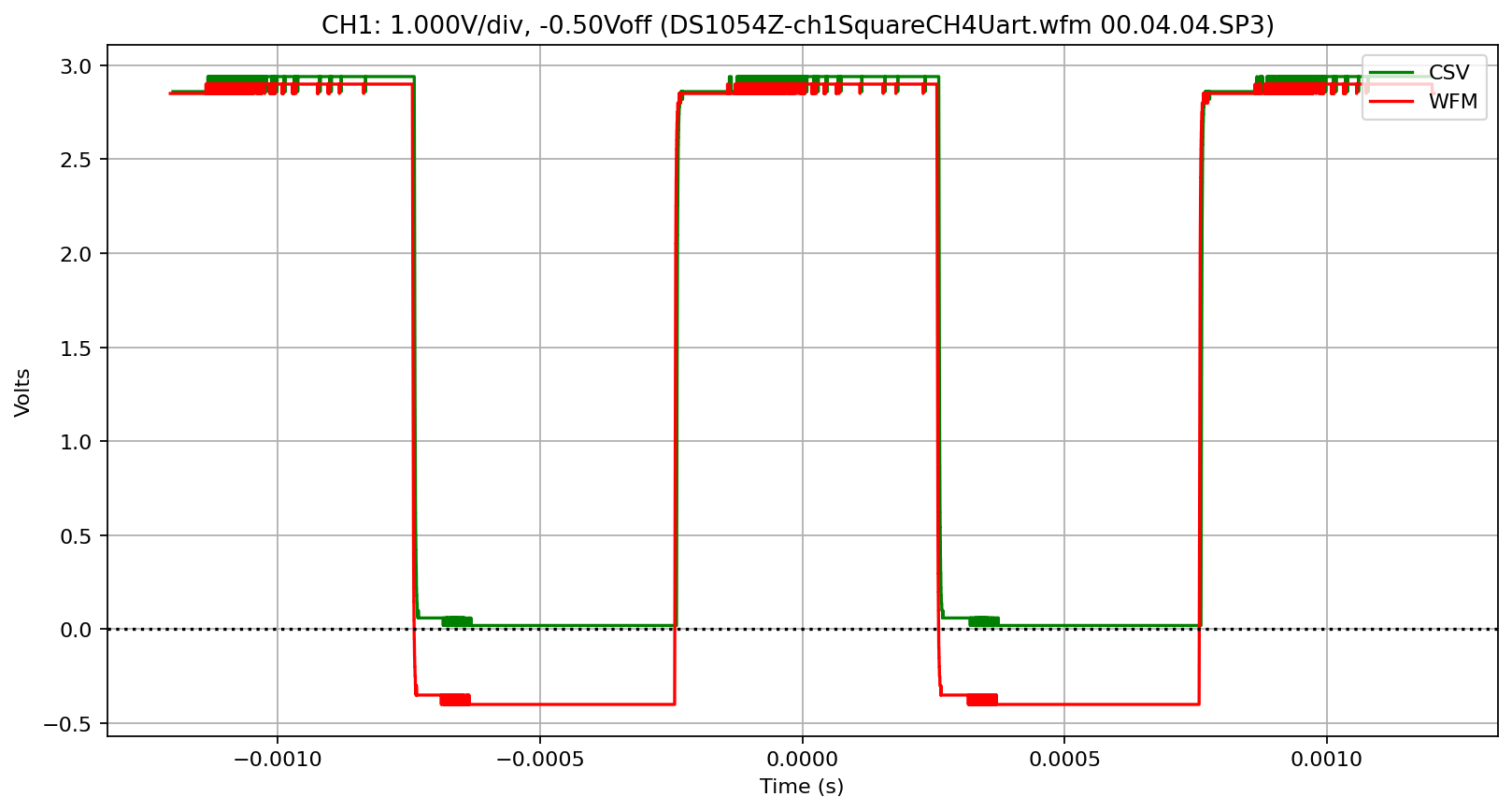
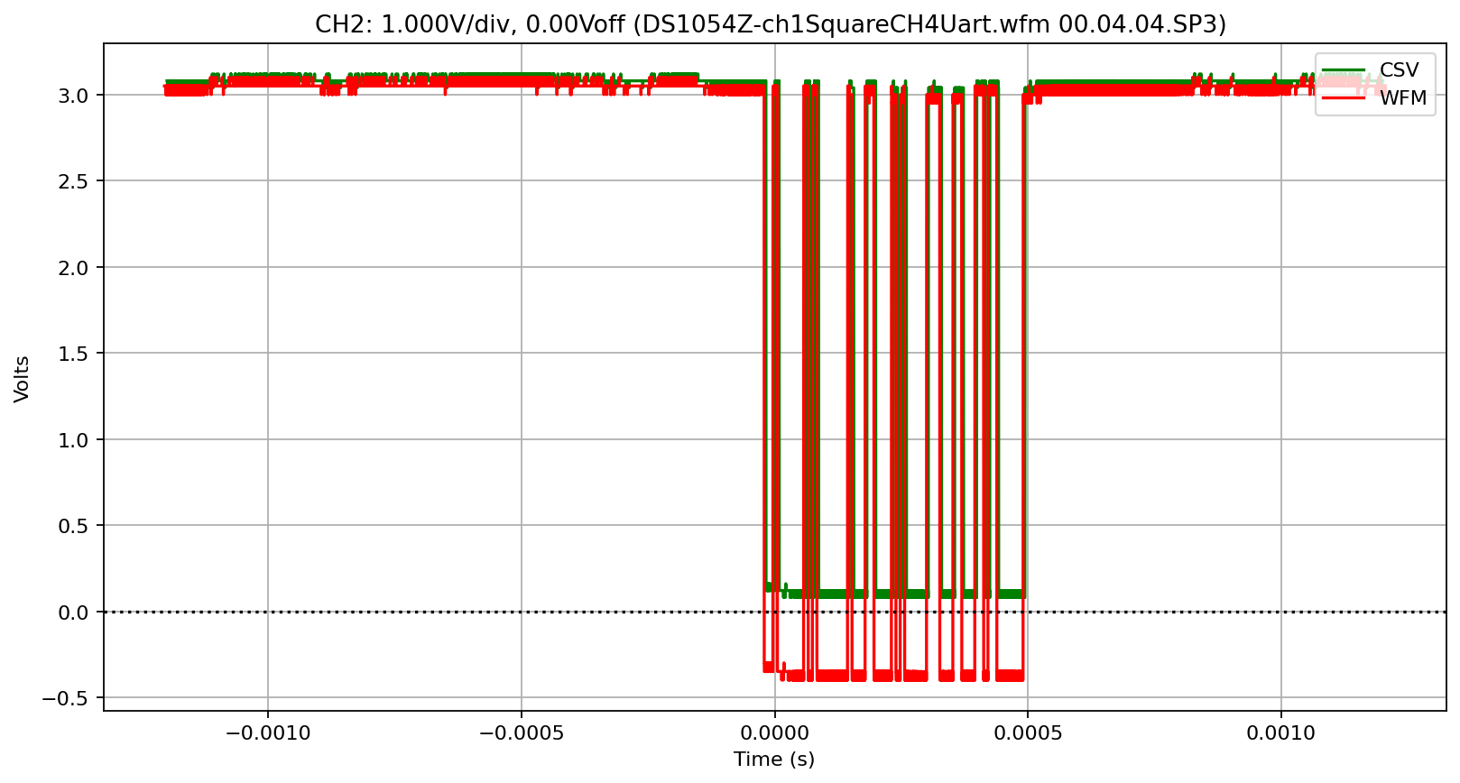
DS1054Z-D Scope file
[Contributed by @wvdv2002](https://github.com/scottprahl/RigolWFM/pull/17)
[24]:
name = "DS1054Z-ch1SquareCH4Uart"
wfm_url = repo + name + ".wfm" + "?raw=true"
w = Wfm.from_url(wfm_url, "1000Z")

csv_filename = repo + name + ".csv"
csv_data = np.genfromtxt(csv_filename, delimiter=",", skip_header=2)
csv_data = csv_data[:, :-1].T

t_incr = 4.000000e-08  # seconds/point
t_start = -len(csv_data[0]) / 2.0 * t_incr  # seconds so that t=0 is in the center
csv_times = csv_data[0] * t_incr + t_start  # seconds

plot_compare(w, csv_times, csv_data, toffset=0)
downloading 'https://raw.githubusercontent.com/scottprahl/RigolWFM/main/tests/files/wfm/DS1054Z-ch1SquareCH4Uart.wfm?raw=true'
[25]:
print(w.describe())
    General:
        File Model   = DS1104Z
        User Model   = 1000Z
        Parser Model = wfm1000z
        Firmware     = 00.04.04.SP3
        Filename     = DS1054Z-ch1SquareCH4Uart.wfm
        Channels     = [1, 4]

    Trigger:
        Derived Level (CH1) = 2.90  V
        Derived Level (CH4) = 3.05  V

     Channel 1:
         Coupling =       DC
            Scale =     1.00  V/div
           Offset =  -500.00 mV
            Probe =      10X
         Inverted =    False

        Time Base =  200.000 µs/div
           Offset =    0.000  s
            Delta =   40.000 ns/point
           Points =    60256

         Count    = [        1,        2,        3  ...     60255,    60256]
           Raw    = [      170,      170,      170  ...       170,      170]
           Times  = [-1.205 ms,-1.205 ms,-1.205 ms  ...  1.205 ms, 1.205 ms]
           Volts  = [  2.85  V,  2.85  V,  2.85  V  ...   2.85  V,  2.85  V]

     Channel 4:
         Coupling =       DC
            Scale =     1.00  V/div
           Offset =     0.00  V
            Probe =      10X
         Inverted =    False

        Time Base =  200.000 µs/div
           Offset =    0.000  s
            Delta =   40.000 ns/point
           Points =    60256

         Count    = [        1,        2,        3  ...     60255,    60256]
           Raw    = [      188,      188,      188  ...       187,      188]
           Times  = [-1.205 ms,-1.205 ms,-1.205 ms  ...  1.205 ms, 1.205 ms]
           Volts  = [  3.05  V,  3.05  V,  3.05  V  ...   3.00  V,  3.05  V]
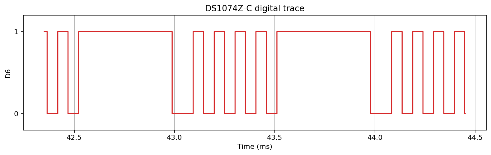
DS1074Z digital channel
DS1074Z-C.wfm is a logic-only capture from a DS1074Z Plus. The parser now exposes the digital trace as D6, and logic_times provides the matching time axis. Plotting a short slice makes the transitions much easier to see than showing all three million points at once.
[26]:
name = "DS1074Z-C"
wfm_url = repo + name + ".wfm" + "?raw=true"
w = Wfm.from_url(wfm_url, "1000Z")

print(w.describe())
downloading 'https://raw.githubusercontent.com/scottprahl/RigolWFM/main/tests/files/wfm/DS1074Z-C.wfm?raw=true'
    General:
        File Model   = DS1074Z Plus
        User Model   = 1000Z
        Parser Model = wfm1000z
        Firmware     = 00.04.05.SP2
        Filename     = DS1074Z-C.wfm
        Channels     = []

    Logic:
        Layout       = interleaved stride 2
        Mapping      = mirrored D7-D0 byte lanes
        Points       =  3000256
        Delta        =   20.000 ns/point
        Traces       = [D6]
        Observed     = [L0.B6, L1.B6]
[27]:
logic_name = "D6"
logic = w.logic_channels[logic_name]
times = w.logic_times

t0 = 42.35e-3
t1 = 44.45e-3
mask = (times >= t0) & (times <= t1)

plt.figure(num=None, figsize=(12, 3), dpi=80, facecolor="w", edgecolor="k")
plt.step(times[mask] * 1e3, logic[mask], where="post", color="tab:red")
plt.ylim(-0.2, 1.2)
plt.yticks([0, 1])
plt.xlabel("Time (ms)")
plt.ylabel(logic_name)
plt.title(f"{name} digital trace")
plt.grid(True, axis="x")
plt.show()