Rigol DS4000 Waveform Examples

Scott Prahl

Mar 2026

import numpy as np
import matplotlib.pyplot as plt
import imageio.v3 as iio

from RigolWFM import Wfm, DS4000_scopes

repo = "https://raw.githubusercontent.com/scottprahl/RigolWFM/main/tests/files/wfm/"

def side_by_png(stem, ch=[1, 2], offset=[0, 0]):
    wfm = Wfm.from_url(repo + stem + ".wfm" + "?raw=true")
    png = iio.imread(repo + stem + ".png" + "?raw=true")

    plt.subplots(2, 1, figsize=(8, 12))

    plt.subplot(211)
    plt.title("Rigol Screenshot")
    plt.imshow(png)
    plt.axis("off")

    plt.subplot(212)

    for channel, off in zip(ch, offset):
        chan = wfm.channels[channel - 1]
        plt.plot(chan.times * 1e6, chan.volts + off, label="CH%d" % channel)

    plt.title(stem + ".wfm (CH1 Top, CH2 Bottom)")
    plt.xlabel("Time (µs)")
    plt.ylabel("Volts (V)")
    plt.ylim(-20, 20)
    plt.legend()
    plt.grid(True)


def side_by_csv(stem, ch2=True, ch2_offset=-15):
    wfm = Wfm.from_url(repo + stem + ".wfm" + "?raw=true")
    csv = np.genfromtxt(repo + stem + ".csv" + "?raw=true", delimiter=",", skip_header=2).T

    plt.subplots(1, 2, figsize=(12, 4.5))

    plt.subplot(121)

    time = -(csv[0, -1] - csv[0, 0]) / 2 + csv[0]
    plt.title(stem + ".csv (CH1 Top, CH2 Bottom)")
    plt.plot(time, csv[1], color="green")
    plt.plot(time, ch2_offset + csv[2], color="red")
    plt.xlabel("Time (µs)")
    plt.ylabel("Volts (V)")
    plt.grid(True)

    plt.subplot(122)

    ch1 = wfm.channels[0]
    plt.plot(ch1.times * 1e6, ch1.volts, color="green")
    plt.title(stem + ".wfm (CH1 Top, CH2 Bottom)")
    if ch2:
        ch = wfm.channels[1]
        plt.plot(ch.times * 1e6, ch2_offset + ch.volts, color="red")
    plt.xlabel("Time (µs)")
    plt.ylabel("Volts (V)")
    plt.grid(True)

A list of Rigol scopes that should have the same file format is:

print(DS4000_scopes)

['4', '4000', 'DS4000', 'DS4054', 'DS4052', 'DS4034', 'DS4032', 'DS4024', 'DS4022', 'DS4014', 'DS4012', 'MSO4054', 'MSO4052', 'MSO4034', 'MSO4032', 'MSO4024', 'MSO4022', 'MSO4014', 'MSO4012']

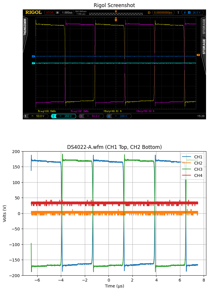
DS4022 Waveform

Compare the .wfm data with screenshot

side_by_png("DS4022-A", ch=[1, 2, 3, 4], offset=[0, 0, 0, 30])
plt.ylim(-200, 200)
plt.show()

downloading 'https://raw.githubusercontent.com/scottprahl/RigolWFM/main/tests/files/wfm/DS4022-A.wfm?raw=true'

DS4024 Waveform

Start with importing the .csv data

filename = "DS4024-A.csv"
csv_filename = repo + filename

csv_data = np.genfromtxt(csv_filename, delimiter=",", skip_header=2).T

# need to do this separately because only the start and increment is given in the csv file
time = csv_data[0] * 2.000000e-06 - 1.400000e-03

Import the .wfm data

# raw=true is needed because this is a binary file
name = "DS4024-A.wfm"
wfm_filename = repo + name + "?raw=true"

w = Wfm.from_url(wfm_filename, "4")

downloading 'https://raw.githubusercontent.com/scottprahl/RigolWFM/main/tests/files/wfm/DS4024-A.wfm?raw=true'

Now describe the .wfm data

print(w.describe())

    General:
        File Model   = DS4A200500078
        User Model   = 4
        Parser Model = wfm4000
        Firmware     = 00.02.03.02.00
        Filename     = DS4024-A.wfm
        Channels     = [1, 2]

    Trigger:
        Derived Level (CH1) = 13.50 mV
        Derived Level (CH2) = -6.25 mV

     Channel 1:
         Coupling =       DC
            Scale =     1.00  V/div
           Offset =  -576.00 mV
            Probe =       1X
         Inverted =    False

        Time Base =  200.000 µs/div
           Offset =  100.000 µs
            Delta =    4.000 ns/point
           Points =   700000

         Count    = [        1,        2,        3  ...    699999,   700000]
           Raw    = [      109,      109,      109  ...       205,      206]
           Times  = [-1.300 ms,-1.300 ms,-1.300 ms  ...  1.500 ms, 1.500 ms]
           Volts  = [ 13.50 mV, 13.50 mV, 13.50 mV  ...   3.01  V,  3.04  V]

     Channel 2:
         Coupling =       DC
            Scale =   200.00 mV/div
           Offset =     0.00  V
            Probe =       1X
         Inverted =    False

        Time Base =  200.000 µs/div
           Offset =  100.000 µs
            Delta =    4.000 ns/point
           Points =   700000

         Count    = [        1,        2,        3  ...    699999,   700000]
           Raw    = [      126,      127,      127  ...       127,      127]
           Times  = [-1.300 ms,-1.300 ms,-1.300 ms  ...  1.500 ms, 1.500 ms]
           Volts  = [ -6.25 mV, -0.00  V, -0.00  V  ...  -0.00  V, -0.00  V]

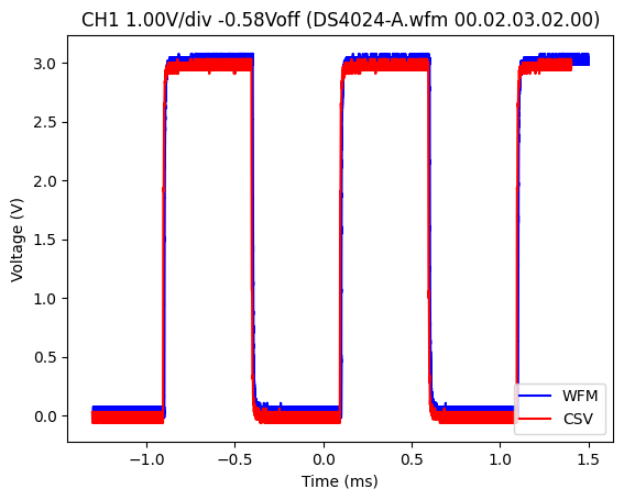
Finally compare the .wfm data to the .csv data

toff = 0.05
ch = w.channels[0]
plt.title("CH%d %.2fV/div %.2fVoff (%s %s)" % (1, ch.volt_per_division, ch.volt_offset, w.basename, w.firmware))
plt.plot(ch.times * 1e3, ch.volts, color="blue", label="WFM")

plt.plot(time * 1e3 + toff, csv_data[1], color="red", label="CSV")
plt.legend(loc="lower right")
plt.xlabel("Time (ms)")
plt.ylabel("Voltage (V)")

plt.show()