Exporting Waveforms as WAV Files for LTspice
Scott Prahl
Mar 2026
[1]:
%config InlineBackend.figure_format = 'retina'

import os
import matplotlib.pyplot as plt
from RigolWFM import Wfm

repo = "https://raw.githubusercontent.com/scottprahl/RigolWFM/main/tests/files/wfm/"
Introduction
A measured waveform captured on a Rigol oscilloscope can be exported as a .wav file and used directly as a voltage or current source in an LTspice simulation. This lets you drive a simulated circuit with a real measured signal — a captured input pulse, a noisy power rail, or an RF envelope — without having to hand-fit a piecewise-linear (PWL) approximation.
The advantages of .wav over .txt/PWL are:
Compact — 2 bytes per sample versus ~20 bytes per line of PWL text (10× smaller)
Fast to load — binary format, no text parsing in LTspice
Multi-channel — a single stereo WAV file can carry two independent signals
WAV File Format
RigolWFM writes signed 16-bit PCM WAV files (the standard CD-audio sample format). Each sample is a 16-bit integer in the range −32767 to +32767. LTspice normalises this range to [−1, +1] and then multiplies by Vpeak to recover physical voltages.
Voltage Scaling
The scale parameter controls how scope voltages are mapped to integers:
|
Mapping |
LTspice |
|---|---|---|
|
signal min → −32767, signal max → +32767 |
|
|
−4×V/div → −32767, +4×V/div → +32767; zero stays at zero |
|
Use "auto" when only the shape matters (e.g. a frequency-domain stimulus). Use "scope" when the DC level is important and you want zero volts to remain zero in the simulation.
Mono vs. Stereo
A mono WAV carries one channel; a stereo WAV carries two, interleaved as left/right audio frames. LTspice selects the channel with the chan= parameter (zero-based: chan=0 = first channel, chan=1 = second).
Using a WAV File in LTspice
Voltage and current sources in LTspice accept a wavefile= attribute:
Vxxx  n+  n-  wavefile="<filename>"  [chan=<n>]  Vpeak=<volts>
Ixxx  n+  n-  wavefile="<filename>"  [chan=<n>]  Vpeak=<amps>
<filename>is an absolute path, or a relative path from the schematic directory.chan=selects the channel (default 0). Only meaningful for stereo files.Vpeakscales the normalised [−1, +1] range to physical units.This source is only active during a
.trananalysis.
Example: RC Low-Pass Filter Driven by a Measured Waveform
Suppose you have captured a noisy 5 kHz square wave on CH1 (2 V/div) and saved it as signal.wav using scale="scope" (so Vpeak = 4 × 2 = 8 V):
* RC low-pass filter - input from measured waveform
V1  in  0  wavefile="signal.wav"  Vpeak=8
R1  in  out  1k
C1  out  0   10n
.tran  0  3.3ms
.backanno
.end
To add the source in the LTspice GUI: right-click the voltage source → Advanced → in the “Value” field enter wavefile="signal.wav" Vpeak=8.
Example: Two-Channel Stimulus from a Stereo WAV
If the .wav was saved with channel=[1, 2], both scope channels live in one file:
* Two independent stimulus signals from one stereo WAV
V1  sig1  0  wavefile="stereo.wav"  chan=0  Vpeak=8
V2  sig2  0  wavefile="stereo.wav"  chan=1  Vpeak=20
API Reference
wfm.wav(filename, *, channel=1, scale="auto")
``filename`` — output path (string,
os.PathLike, or a writable binary file object)``channel`` — scope channel number(s) to export. An
intgives a mono file; a two-elementlistgives a stereo file (e.g.[1, 2]).``scale`` —
"auto"or"scope"(see table above)
A ValueError is raised if more than two channels are specified or if a requested channel is missing, not enabled, or not selected.
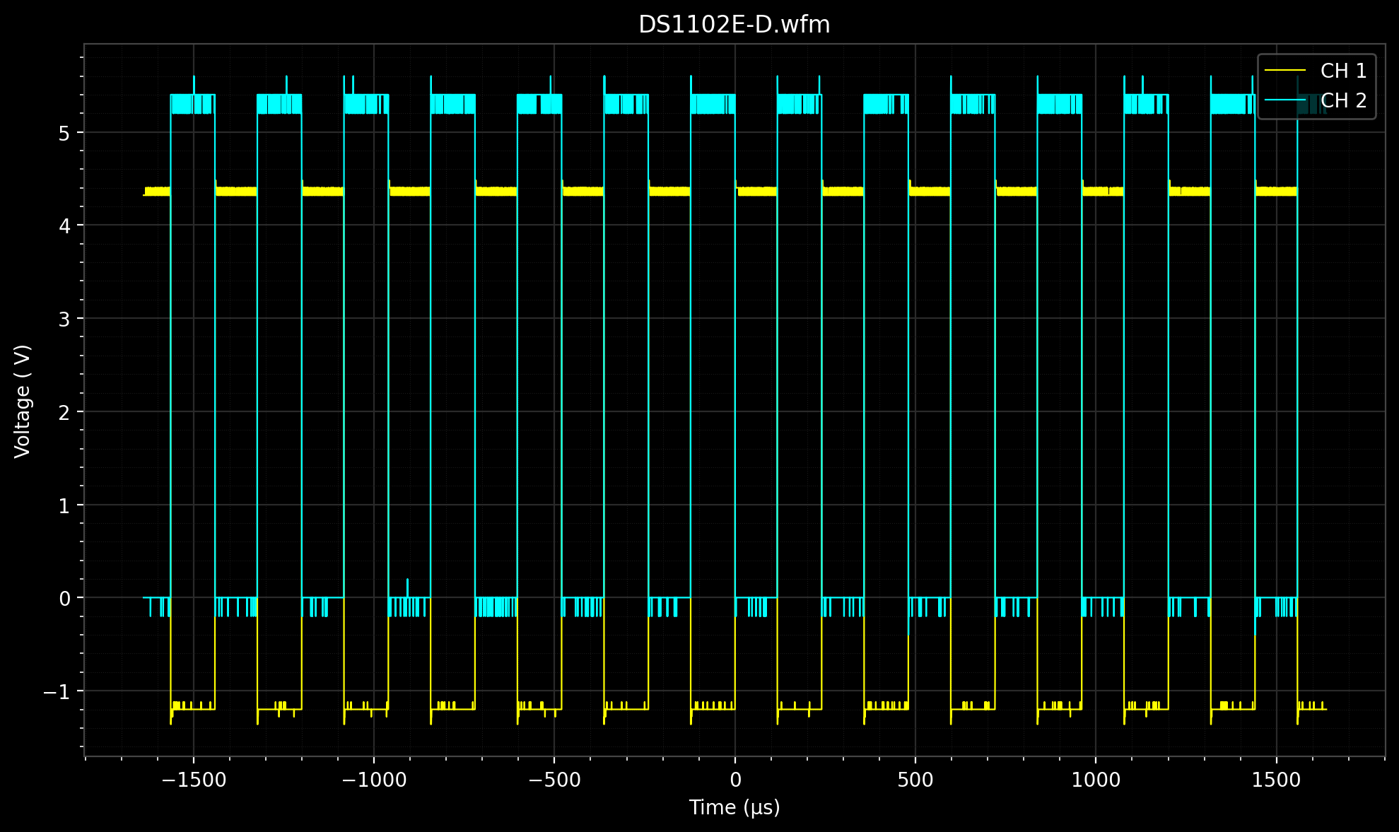
Example Waveform
Load a two-channel DS1102E capture from the project repository.
[2]:
stem = "DS1102E-D"
w = Wfm.from_url(repo + stem + ".wfm?raw=true", "E")
print(w.describe())
    General:
        File Model   = DS1000E
        User Model   = E
        Parser Model = wfm1000e
        Firmware     = unknown
        Filename     = DS1102E-D.wfm
        Channels     = [1, 2]

    Trigger:
        Mode     = edge
        Source   = CH1
        Level    = 1.60  V
        Sweep    = AUTO
        Coupling = DC
        Derived Level     = -1.20  V

     Channel 1:
         Coupling =  unknown
            Scale =     2.00  V/div
           Offset =     2.40  V
            Probe =       1X
         Inverted =    False

        Time Base =  100.000 µs/div
           Offset =    0.000  s
            Delta =  400.000 ns/point
           Points =     8192

         Count    = [        1,        2,        3  ...      8191,     8192]
           Raw    = [       41,       41,       41  ...       110,      110]
           Times  = [-1.638 ms,-1.638 ms,-1.638 ms  ...  1.638 ms, 1.638 ms]
           Volts  = [  4.32  V,  4.32  V,  4.32  V  ...  -1.20  V, -1.20  V]

     Channel 2:
         Coupling =  unknown
            Scale =     5.00  V/div
           Offset =   -15.80  V
            Probe =       1X
         Inverted =    False

        Time Base =  100.000 µs/div
           Offset =    0.000  s
            Delta =  400.000 ns/point
           Points =     8192

         Count    = [        1,        2,        3  ...      8191,     8192]
           Raw    = [      204,      204,      204  ...       178,      178]
           Times  = [-1.638 ms,-1.638 ms,-1.638 ms  ...  1.638 ms, 1.638 ms]
           Volts  = [  0.00  V,  0.00  V,  0.00  V  ...   5.20  V,  5.20  V]
downloading 'https://raw.githubusercontent.com/scottprahl/RigolWFM/main/tests/files/wfm/DS1102E-D.wfm?raw=true'
[3]:
w.plot()
plt.show()
Mono WAV — scale="auto"
The signal’s own voltage range is mapped to ±32767. The waveform shape is preserved but the DC level is lost. To reconstruct the original amplitude in LTspice, set Vpeak to half the peak-to-peak voltage of the signal.
For CH1 in this capture the voltage swings from about −1.36 V to 4.48 V, so the peak-to-peak is ≈ 5.84 V and Vpeak ≈ 2.92 V.
[4]:
import numpy as np

ch1 = next(c for c in w.channels if c.channel_number == 1)
v_min, v_max = float(np.min(ch1.volts)), float(np.max(ch1.volts))
vpeak_auto = (v_max - v_min) / 2
print(f"CH1 voltage range: {v_min:.3f} V  to  {v_max:.3f} V")
print(f"LTspice Vpeak for scale='auto': {vpeak_auto:.3f} V")

wav_auto = stem + "_auto.wav"
w.wav(wav_auto, channel=1, scale="auto")
print(f"Written: {wav_auto}  ({os.path.getsize(wav_auto)} bytes)")
CH1 voltage range: -1.360 V  to  4.480 V
LTspice Vpeak for scale='auto': 2.920 V
Written: DS1102E-D_auto.wav  (16428 bytes)
LTspice netlist entry for this file:
V1 in 0 wavefile="DS1102E-D_auto.wav" Vpeak=2.92
Mono WAV — scale="scope"
The scope’s full-scale range (±4 × V/div) is mapped to ±32767. Zero volts stays at zero, so the DC level is preserved. Set Vpeak = 4 × V/div in LTspice.
CH1 is set to 2 V/div, so the full-scale range is ±8 V and Vpeak = 8 V.
[5]:
vpeak_scope = 4 * ch1.volt_per_division
print(f"CH1 V/div: {ch1.volt_per_division:.2f} V")
print(f"LTspice Vpeak for scale='scope': {vpeak_scope:.2f} V")

wav_scope = stem + "_scope.wav"
w.wav(wav_scope, channel=1, scale="scope")
print(f"Written: {wav_scope}  ({os.path.getsize(wav_scope)} bytes)")
CH1 V/div: 2.00 V
LTspice Vpeak for scale='scope': 8.00 V
Written: DS1102E-D_scope.wav  (16428 bytes)
LTspice netlist entry for this file:
V1 in 0 wavefile="DS1102E-D_scope.wav" Vpeak=8
Stereo WAV — Two Channels in One File
Pass a two-element list to channel to write both scope channels into a single stereo WAV. In LTspice, chan=0 selects CH1 and chan=1 selects CH2.
[6]:
ch2 = next(c for c in w.channels if c.channel_number == 2)
vpeak_ch1 = 4 * ch1.volt_per_division
vpeak_ch2 = 4 * ch2.volt_per_division
print(f"CH1 V/div = {ch1.volt_per_division:.2f} V  →  Vpeak = {vpeak_ch1:.2f} V")
print(f"CH2 V/div = {ch2.volt_per_division:.2f} V  →  Vpeak = {vpeak_ch2:.2f} V")

wav_stereo = stem + "_stereo.wav"
w.wav(wav_stereo, channel=[1, 2], scale="scope")
print(f"Written: {wav_stereo}  ({os.path.getsize(wav_stereo)} bytes)")
CH1 V/div = 2.00 V  →  Vpeak = 8.00 V
CH2 V/div = 5.00 V  →  Vpeak = 20.00 V
Written: DS1102E-D_stereo.wav  (32812 bytes)
LTspice netlist entries for the stereo file:
V1  sig1  0  wavefile="DS1102E-D_stereo.wav"  chan=0  Vpeak=8
V2  sig2  0  wavefile="DS1102E-D_stereo.wav"  chan=1  Vpeak=20
Command-Line Usage
The wfmconvert command-line tool can also produce WAV files. The --channel flag selects one or two channels; --scale sets the voltage mapping.
# Mono WAV from CH1, auto scaling
wfmconvert --channel 1 wav DS1102E-D.wfm

# Mono WAV from CH1, scope scaling
wfmconvert --channel 1 --scale scope wav DS1102E-D.wfm

# Stereo WAV from CH1 and CH2 using scope scaling
wfmconvert --channel 12 --scale scope wav DS1102E-D.wfm
[7]:
# Clean up generated WAV files
for f in [wav_auto, wav_scope, wav_stereo]:
    if os.path.exists(f):
        os.remove(f)