RigolWFM Quick Start
Scott Prahl
Apr 2026
This notebook shows the shortest useful path through RigolWFM: load a waveform, inspect what was parsed, work with the sample arrays, and plot the result.
Install
pip install RigolWFM
Most of the time you can let the library auto-detect the waveform family. Pass model= only when you want to override detection or when you already know the scope family.
[1]:
%config InlineBackend.figure_format = 'retina'

import os
import tempfile

os.environ.setdefault("MPLCONFIGDIR", tempfile.mkdtemp())

import matplotlib.pyplot as plt

from RigolWFM import Wfm

repo = "https://raw.githubusercontent.com/scottprahl/RigolWFM/main/tests/files/"


def sample_url(relative_path: str) -> str:
    return repo + relative_path
1. Load a Sample Waveform
The docs notebooks always use real sample files from the GitHub repo. Here we load a two-channel DS1102E capture directly from a raw GitHub URL.
[2]:
w = Wfm.from_url(sample_url("wfm/DS1102E-D.wfm"))
w
downloading 'https://raw.githubusercontent.com/scottprahl/RigolWFM/main/tests/files/wfm/DS1102E-D.wfm'
[2]:
<RigolWFM.wfm.Wfm at 0x11488a3c0>
2. See What Was Parsed
A quick summary is usually enough to confirm that the right file, parser, and channels were found. Use w.describe() when you want the full scope settings and channel metadata dump.
[3]:
print("Scope reported by file header :", w.header_name)
print("Parser used                 :", w.parser_name)
print("Enabled analog channels     :", [ch.name for ch in w.channels])
print("Points in first channel     :", len(w.channels[0].volts))
Scope reported by file header : DS1000E
Parser used                 : wfm1000e
Enabled analog channels     : ['CH 1', 'CH 2']
Points in first channel     : 8192
[4]:
print(w.describe())
    General:
        File Model   = DS1000E
        User Model   = auto
        Parser Model = wfm1000e
        Firmware     = unknown
        Filename     = DS1102E-D.wfm
        Channels     = [1, 2]

    Trigger:
        Mode     = edge
        Source   = CH1
        Level    = 1.60  V
        Sweep    = AUTO
        Coupling = DC
        Derived Level     = -1.20  V

     Channel 1:
         Coupling =  unknown
            Scale =     2.00  V/div
           Offset =     2.40  V
            Probe =       1X
         Inverted =    False

        Time Base =  100.000 µs/div
           Offset =    0.000  s
            Delta =  400.000 ns/point
           Points =     8192

         Count    = [        1,        2,        3  ...      8191,     8192]
           Raw    = [       41,       41,       41  ...       110,      110]
           Times  = [-1.638 ms,-1.638 ms,-1.638 ms  ...  1.638 ms, 1.638 ms]
           Volts  = [  4.32  V,  4.32  V,  4.32  V  ...  -1.20  V, -1.20  V]

     Channel 2:
         Coupling =  unknown
            Scale =     5.00  V/div
           Offset =   -15.80  V
            Probe =       1X
         Inverted =    False

        Time Base =  100.000 µs/div
           Offset =    0.000  s
            Delta =  400.000 ns/point
           Points =     8192

         Count    = [        1,        2,        3  ...      8191,     8192]
           Raw    = [      204,      204,      204  ...       178,      178]
           Times  = [-1.638 ms,-1.638 ms,-1.638 ms  ...  1.638 ms, 1.638 ms]
           Volts  = [  0.00  V,  0.00  V,  0.00  V  ...   5.20  V,  5.20  V]
3. Work With the Sample Arrays
Each enabled analog channel is available as a Channel object in w.channels. The main arrays you will usually use are times, volts, and raw.
[5]:
ch1 = w.channels[0]

print("Channel name:", ch1.name)
print("First five times (s):", ch1.times[:5])
print("First five volts (V):", ch1.volts[:5])
print("First five raw ADC counts:", ch1.raw[:5])
Channel name: CH 1
First five times (s): [-0.0016384 -0.001638  -0.0016376 -0.0016372 -0.0016368]
First five volts (V): [4.32 4.32 4.32 4.32 4.32]
First five raw ADC counts: [41 41 41 41 41]
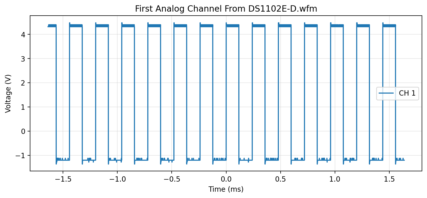
[6]:
fig, ax = plt.subplots(figsize=(10, 4))
ax.plot(ch1.times * 1e3, ch1.volts, label=ch1.name)
ax.set_xlabel("Time (ms)")
ax.set_ylabel("Voltage (V)")
ax.set_title("First Analog Channel From DS1102E-D.wfm")
ax.grid(True, alpha=0.3)
ax.legend()
plt.show()
4. Quick Text Export Preview
Wfm.csv() returns a CSV-formatted string. The dedicated export notebooks go deeper, but a quick preview is handy when you just want to confirm the X axis and channel columns.
[7]:
rows = w.csv().splitlines()
for row in rows[:4]:
    print(row)
X,CH 1,CH 2,Start,Increment
µs, V, V,-1638.3999999999999,0.39999999999999997
-1638.3999999999999,4.32,0.00
-1637.9999999999998,4.32,0.00
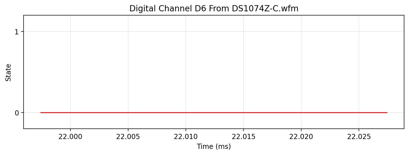
5. Digital Channels Are Exposed Separately
If a waveform file contains parsed logic data, those traces appear in logic_channels. Here is the simplest Z-series example in the repo, which exposes D6.
[8]:
logic = Wfm.from_url(sample_url("wfm/DS1074Z-C.wfm"), model="Z")
sorted(logic.logic_channels)
downloading 'https://raw.githubusercontent.com/scottprahl/RigolWFM/main/tests/files/wfm/DS1074Z-C.wfm'
[8]:
['D6']
[9]:
d6 = logic.logic_channels["D6"]
t = logic.logic_times

fig, ax = plt.subplots(figsize=(10, 3))
ax.step(t[:1500] * 1e3, d6[:1500], where="post", color="tab:red")
ax.set_xlabel("Time (ms)")
ax.set_ylabel("State")
ax.set_yticks([0, 1])
ax.set_ylim(-0.2, 1.2)
ax.set_title("Digital Channel D6 From DS1074Z-C.wfm")
ax.grid(True, alpha=0.3)
plt.show()
6. Local Files and Channel Selection
When you already have a waveform on disk, use Wfm.from_file(...):
from RigolWFM import Wfm

w = Wfm.from_file('/path/to/capture.wfm')
ch1_only = Wfm.from_file('/path/to/capture.wfm', selected='1')
The selected string filters analog channels 1 through 4 before plotting or export.
Where To Go Next
the family notebooks such as DS1000E Waveforms when you want model-specific examples